
這篇筆記整理了 ICCV 2023 的 Ref-NeuS 論文。該研究針對多視角影像中帶有反射的物體重建問題,提出了一個減少歧異性的神經隱式表面學習框架,旨在解決反射導致的多視角不一致性與模糊問題。論文提出一個專門處理反射表面的方法,其核心技術包括:透過分析多視角顏色不一致性和點的可見性來定義「反射分數」,以此識別反射區域;設計一個「反射感知光度損失」,根據反射分數自適應地降低反射像素的權重;以及利用反射方向來建構更精確的輻射場。實驗結果顯示,相較於現有方法,Ref-NeuS 在具有反射的場景中,能夠重建出更高品質的表面幾何、更平滑的表面法線,並維持良好的渲染效果。
論文資訊
- Link: https://arxiv.org/abs/2303.10840
- Conference: ICCV 2023
Introduction#
Problem Setting
- 反射區域的多視圖不一致性,導致重建結果模糊。
Reasons 作者認為反射表面的模糊原因如下:
- 反射區域的重建幾何不準確。
- 反射區域的多視圖不一致。
Purpose
- 透過減弱反射表⾯的影響來減少模糊性。
Previous Works and Challenges
- NeRF 和 NeuS:對於具有反射的物體,會產生模糊的結果。
- Ref-NeRF 和 Neural-Warp:雖然可以透過以反射方向取代入射方向改善生成品質,但是無法產生平滑的表面法向量,因此提升效果有限。
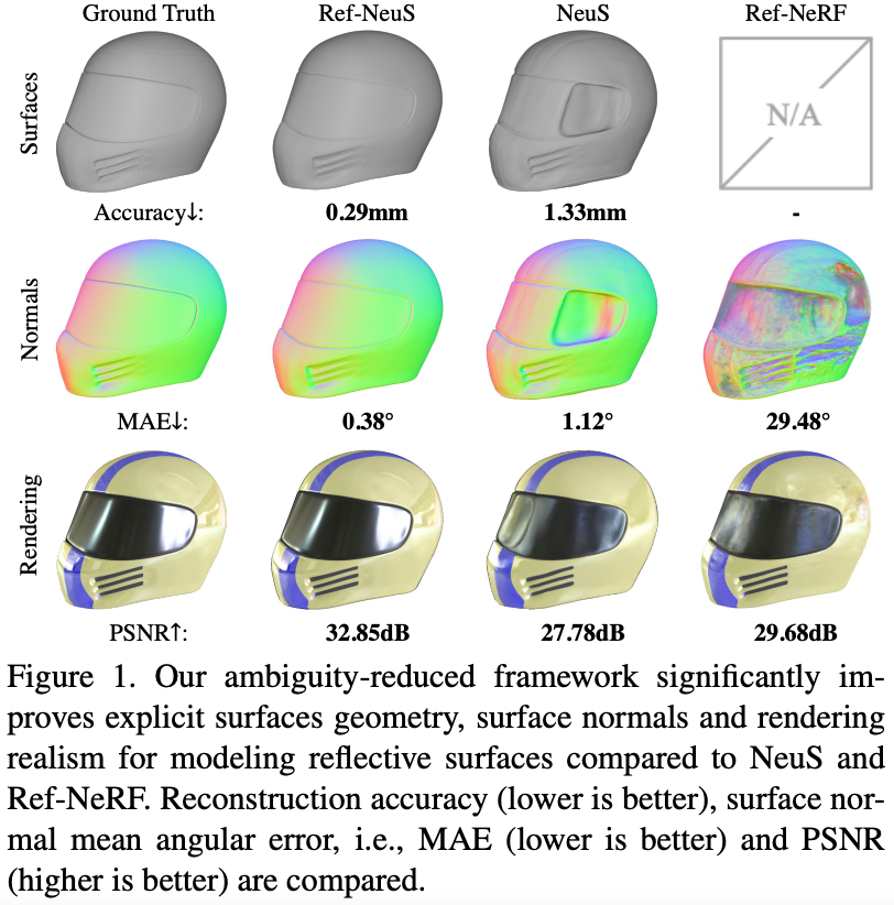
Figure 1 Contribution
- 提出了第⼀個⽤於重建具有反射表⾯的物體的神經隱式表⾯學習框架。
- 使神經隱式表⾯學習能夠處理反射表⾯,以產⽣⾼品質的表⾯幾何形狀和表⾯法線。
- 實驗表明,所提出的框架明顯優於反射表⾯上最先進的⽅法。
Methods#
Overview#
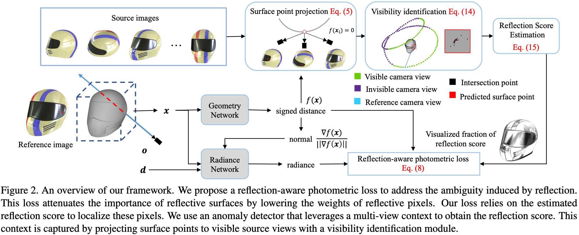
Geometry Network 與 Radiance Network 是使用與 NeuS 相同的架構。
- 將圖像輸入 Geometry Network 以預測用來表示表面的 SDF。
- 使用 SDF 計算表面的法向量,並將法向量與 view direction 一同輸入 Radiance Network,預測 radiance。
- SDF 同時也會計算每個點的可見度與反射分數 (不可見的點沒有計算反射分數的意義)。
- 最後,在計算 reflection-aware photometric loss 時,除了 radiance, SDF ,還會使用反射分數進行約束。
Volume Rendering with Implicit Surface#
在 NeRF 中通過 volume rendering 來計算每個像素最終的顏色:
$$ \begin{align*} \hat{\mathbf{C}}(\mathbf{r}) = \sum_{i=1}^{P} T_i \alpha_i \mathbf{c}_i, \tag{1} \label{eq:1} \end{align*} $$$$ \begin{align*} T_i &= \exp \left( -\sum_{j=1}^{i-1} \alpha_j \delta_j \right) \\ \alpha_i &= 1 - \exp \left( -\sigma_i \delta_i \right) \end{align*} $$使用 MSE Loss 計算預測顏色與 ground-truth 之間的誤差:
$$ \begin{align*} \mathcal{L}_{\text{color}} = \sum_{\mathbf{r} \in \mathcal{R}} \| \mathbf{C}(\mathbf{r}) - \hat{\mathbf{C}}(\mathbf{r}) \|_2^2 \tag{2} \label{eq:2} \end{align*} $$然而,density-based volume rendering 缺乏對於表面的明確定義,因此無法準確提取表面。
而 NeuS 將 3D 場景表示成 signed distance 與 radiance:
$$ \begin{align*} s = f(\mathbf{x}), \quad \mathbf{c} = c(\mathbf{x}, \mathbf{d}), \tag{3} \label{eq:3} \end{align*} $$其中 Geometry Network $f$ 會將空間位置映射到對應的 signed distance $f(\mathbf{x})$,而 Radiance Network $c$ 以位置與 viewing direction 為條件,預測顏色,來建構 view-dependent radiance。
因此 volume rendering 過程中, $\alpha_i$ 是通過 signed distance 計算得到,而非 NeRF 中的 density:
$$ \begin{align*} \alpha_i = \max \left( \frac{\Phi_s(f(\mathbf{x}_i)) - \Phi_s(f(\mathbf{x}_{i+1}))}{\Phi_s(f(\mathbf{x}_i))}, 0 \right), \tag{4} \end{align*} $$$$ \begin{align*} \Phi_s(x) = (1+e^{-sx})^{-1} \end{align*} $$| 符號 | 描述 |
|---|---|
| $1/s$ | A trainable parameter which indicates the standard deviation of $\Phi_s(x)$. |
Anomaly Detection for Reflection Score#
對於多視圖重建任務,多視圖一致性是精確表面重建的保證。然而,對於反射像素會破壞多視圖一致性。
為了克服這個問題,作者提出透過 reflection-aware photometric loss 來減少反射表面的影響,他會自適應地降低分配給反射像素的權重。
為了實現這一點,需要定義反射分數使我們能夠辨識反射像素。
一個簡單的解決方案是參考 NeRF-W [27] 中定義的不確定性視為反射分數。此方法將場景的輻射值建模為高斯分佈,並將預測的不確定性視為變異數。然而,該方法的 MLP 學習到的隱含不確定性是在單一射線上定義的,沒有考慮多視圖上下文,因此無法準確定位反射表面。
作者參考 NeRF-W 中將光線顏色渲染為高斯分佈 $\hat{\mathbf{C}}(\mathbf{r}) \sim (\bar{\mathbf{C}}(\mathbf{r}), \bar{\beta}^2(\mathbf{r}))$ 的做法。
- 平均值 $\bar{\mathbf{C}}(\mathbf{r})$:使用 Eq. \eqref{eq:1} 來查詢。
- 變異數 $\bar{\beta}^2(\mathbf{r})$:利用同一表面點的多視圖像素顏色來確定變異數。
為了獲得多視圖的像素顏色,作者將表面點 $\mathbf{x}$ 投影到不同視圖 $\{ \mathbf{I}_i \}^N_{i=1}$ 上,並使用雙線性插值取得對應的像素顏色 $\{ \mathbf{C}_i (\mathbf{r}) \}^N_{i=1}$。整個投影並獲取像素顏色的過程可以表示成 Eq. \eqref{eq:5}:
$$ \begin{align*} \mathcal{G} &= \mathbf{K} \cdot (\mathbf{R} \cdot \mathbf{x} + \mathbf{T}), \tag{5} \label{eq:5} \\ \mathbf{C} &= \text{interp}(\mathbf{I}, \mathcal{G}), \end{align*} $$| 符號 | 描述 |
|---|---|
| $\mathbf{K}$ | The internal calibration matrix. |
| $\mathbf{R}$ | The rotation matrix. |
| $\mathbf{T}$ | The translate matrix. |
| $\cdot$ | The matrix multiplication. |
由於只有部分區域包含反射,因此作者將反射定義為異常檢測問題,期望反射表面被視為異常並分配高反射分數。
作者使用 Mahalanobis distance 來作為反射分數(其實就是變異數):
$$ \begin{align*} \bar{\beta}_i^2(\mathbf{r}) = \gamma \frac{1}{N} \sum_{j=1}^{N} \sqrt {\left( \mathbf{C}(\mathbf{r}) - \mathbf{C}_j(\mathbf{r}) \right)^T \Sigma^{-1} \left( \mathbf{C}_i(\mathbf{r}) - \mathbf{C}_j(\mathbf{r}) \right)}, \tag{6} \label{eq:6} \end{align*} $$| 符號 | 描述 |
|---|---|
| $\gamma$ | The scale factor to control the scale of the reflection score. |
| $\Sigma$ | The empirical covariance matrix. |
有了上面的反射分數,我們就可以通過最小化 ray distribution 的負對數似然來將前面提到的 Eq. \eqref{eq:2} 擴展為 reflection-aware photometric loss :
$$ \begin{align*} \mathcal{L}_{\text{color}} = -\log p(\hat{\mathbf{C}}(\mathbf{r})) = \sum_{\mathbf{r} \in \mathcal{R}} \frac{\| \mathbf{C}(\mathbf{r}) - \bar{\mathbf{C}}(\mathbf{r}) \|_2^2}{2{\bar{\beta}}^2(\mathbf{r})} + \frac{\log {\bar{\beta}}^2(\mathbf{r})}{2}. \tag{7} \end{align*} $$由於 ${\bar{\beta}}^2$ 是由 Eq. \eqref{eq:6} 計算的,因此可以將其視為一個常數,並從目標函數中移出。
此外根據以往的多視圖重建任務,我們使用 L1 Loss 來取代 L2 Loss。
因此,最終的 reflection-aware photometric loss 可以表示成 Eq. \eqref{eq:8}:
{% raw %}
$$ \begin{align*} \mathcal{L}_{\text{color}} = \sum_{\mathbf{r} \in \mathcal{R}} \frac{|\mathbf{C}(\mathbf{r}) - \bar{\mathbf{C}}(\mathbf{r})|}{{\bar{\beta}}^2(\mathbf{r})}. \tag{8} \label{eq:8} \end{align*} $${% endraw %}
這邊要注意,作者提到 Eq. \eqref{eq:8} 中的 ${\bar{\beta}}^2$ 只是要表示一個關係,但實際上需要根據 L2 → L1 作相應的調整。
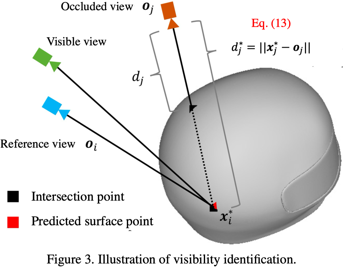
Visibility Identification for Reflection Score#
由於自遮擋,某些像素實際上並不可見,因此在計算反射分數的時候不需要被考慮。
首先,先定義表面:
$$ \begin{align*} \hat{S}_i = \{\mathbf{x} | f(\mathbf{x}) = 0\}. \tag{9} \end{align*} $$由於一條射線上存在無限多個點,因此需要將其離散化。
在離散化之後,如果鄰近兩個採樣點 ($\mathbf{x}_j, \mathbf{x}_{j+1}$) 的符號不同(正負交替),則表示其間隔 $[\mathbf{x}_j, \mathbf{x}_{j+1}]$ 與表面相交:
$$ \begin{align*} T_i = \{\mathbf{x}_j | f(\mathbf{x}_j) \cdot f(\mathbf{x}_{j+1}) < 0\}. \tag{9} \end{align*} $$交點集合 $\hat{S}_i$ 可以透過線性插值得到:
$$ \begin{align*} \hat{S}_i = \left\{ \mathbf{x} | \mathbf{x} = \frac{f(\mathbf{x}_j)\mathbf{x}_{j+1} - f(\mathbf{x}_{j+1})\mathbf{x}_j}{f(\mathbf{x}_j) - f(\mathbf{x}_{j+1})}, \mathbf{x}_j \in T_i \right\}. \tag{11} \end{align*} $$實際上,射線可能與物體在多個表面相交。因此作者只計算第一個交集:
$$ \begin{align*} \mathbf{x}^*_i = \text{argmin } \mathcal{D}(\mathbf{x}, \mathbf{o}_i), \tag{12} \end{align*} $$| 符號 | 描述 |
|---|---|
| $\mathcal{D}(\cdot, \mathbf{o}_i)$ | The distance between point x and the origin of the ray. |
預測的表面點與相機原點的距離可以表示成 Eq. \eqref{eq:13}:
$$ \begin{align*} d_j^* = \|\mathbf{x}_i^* - \mathbf{o}_j\|. \tag{13} \label{eq:13} \end{align*} $$可見性可以表示成:
$$ \begin{align*} v_j = \mathbb{I}(d_j^* \leq d_j). \tag{14} \end{align*} $$| 符號 | 描述 |
|---|---|
| $d_j$ | The distance from the camera location to the first intersection of the intermediate reconstructed mesh by ray casting. |
| $\mathbb{I}(\cdot)$ | The indicator function. |
基於可見性的近似,作者進一步移除了 Eq. \eqref{eq:6} 中不可見的像素,然後微調反射分數計算:
$$ \begin{align*} {\bar{\beta}}^2(\mathbf{r}) &= \gamma \frac{1}{\sum_{j=1}^{N} v_j}\sum_{j=1}^{N} v_j \text{Mdis}, \\ \text{Mdis} &= \sqrt{(\mathbf{C}_i(\mathbf{r}) - \mathbf{C}_j(\mathbf{r}))^T \Sigma^{-1} (\mathbf{C}_i(\mathbf{r}) - \mathbf{C}_j(\mathbf{r}))}. \tag{15} \end{align*} $$作者在 Fig.4 中展示反射分數的可視化結果:
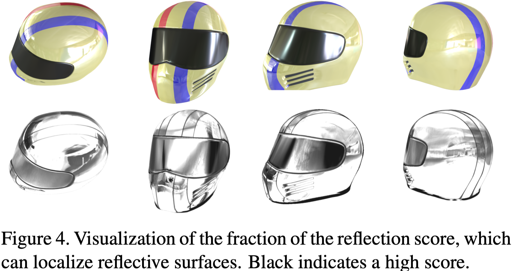
黑色表示高反射區域。
Reflection Direction Dependent Radiance#
遵循 Ref-NeRF 的方式,使用反射向量來獲得更準確的輻射場。
原先的 Eq. \eqref{eq:3} 改寫成:
$$ \begin{align*} \mathbf{c} = c(\mathbf{x}, \mathbf{\hat{d}}), \tag{16} \end{align*} $$Reflection direction 通過 Eq. \eqref{eq:17} 計算得到:
$$ \begin{align*} \mathbf{\hat{d}} = 2(-\mathbf{d} \cdot \mathbf{\hat{n}})\mathbf{\hat{n}} + \mathbf{d}, \tag{17} \label{eq:17} \end{align*} $$表面法向量:
$$ \begin{align*} \mathbf{\hat{n}} = \frac{\nabla f(\mathbf{x})}{\|\nabla f(\mathbf{x})\|}. \tag{18} \end{align*} $$與 Ref-NeRF 相比,由於本篇方法可以產生更好的估計法向量,因此反射方向會更精準,進而產生更準確的輻射場。
Optimization#
Total loss function:
$$ \begin{align*} \mathcal{L} = \mathcal{L}_\text{color} + \alpha \mathcal{L}_\text{eik}. \tag{19} \end{align*} $$$$ \begin{align*} \mathcal{L}_{\text{eik}} = \frac{1}{P} \sum_{i=1}^{P} (|\nabla f(\mathbf{x}_i)| - 1)^2. \tag{20} \end{align*} $$其中 $\mathcal{L}_\text{color}$ 為 reflection-aware photometric loss,而 $\mathcal{L}_{\text{eik}}$ 是用來正規化幾何網路的梯度。
Experiments#
Experimental Settings#
Datasets
- Shiny Blender
- Blender
- SLF
- Bag of Chips
NoteShiny Blender 以外的其他 datasets,作者僅挑選具有光澤的物體。
Metrics
- Chamfer Distance (Acc)
- MAE: 計算法向量誤差。
- PSNR: 計算渲染品質。
Baselines
- IDR
- 多視圖重建
- UNISURF, VolSDF, NeuS
- The warp-based consistency learning methods
- NeuralWarp, Geo-NeuS
- 專⾨為反射物件的重建方法
- Ref-NeRF, PhySG
Implementation Details#
- 基於 NeuS 實現,因此 Geometry Network 與 Radiance Network 與 NeuS 相同。
- 為了實現實時估計可見性,intermediate reconstruction result 會每 500 iter 更新一次,並搭配 128 的解析度來降低計算開銷。 收斂後,可以使用 512 解析度的 Marching Cube 從 SDF 中提取網格。
- 使用單一 RTX 3090 Ti GPU 訓練 7 小時。
Comparison with State-of-the-Art Methods#
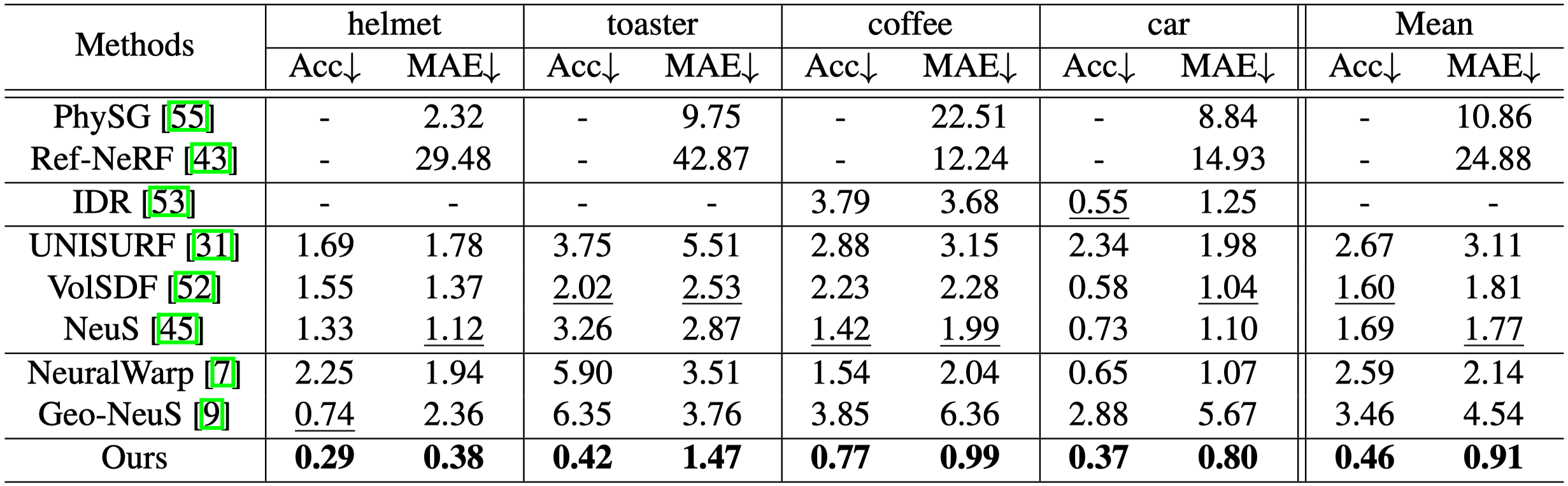
- 由於 COLMAP 與 NeRF-W 無法恢復反射表面,因此沒有與他們比較 Acc。
- PhySG 和 Ref-NeRF 目的為新視角合成,因此論文中沒有展示 Acc。
- IDR 無法為 helmet 與 toaster 產生有意義的重建,因此作者只展示 coffee 與 car。
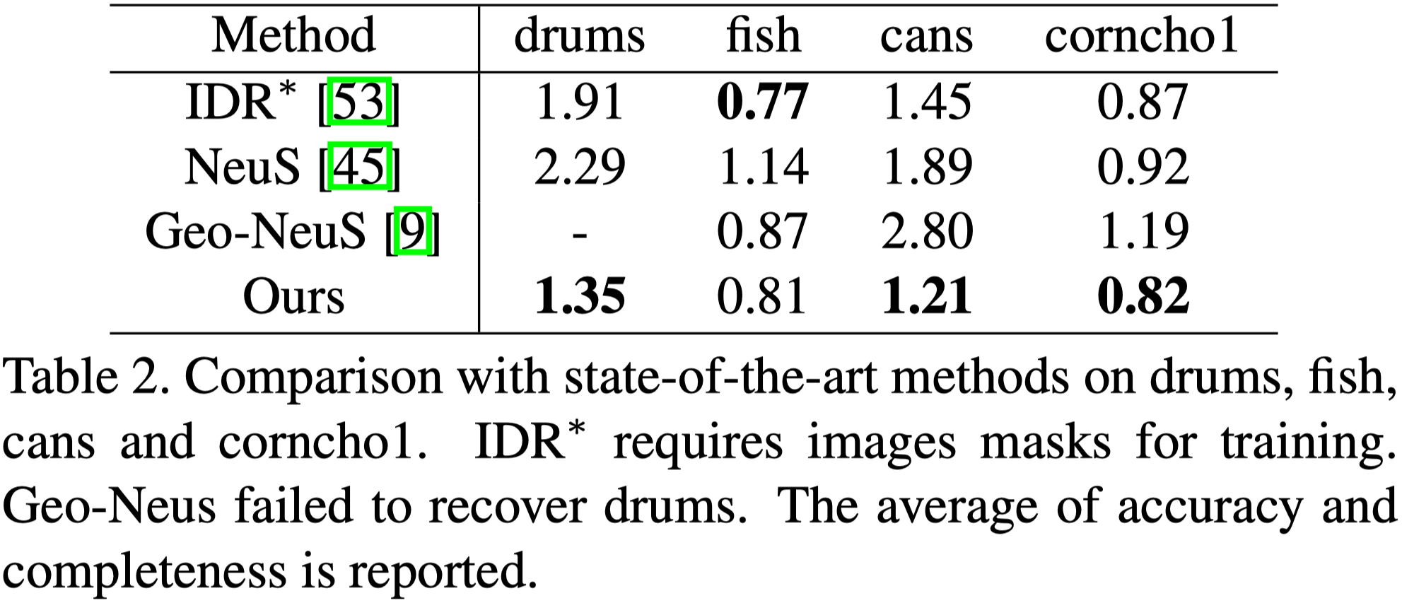
- 本篇的方法明顯優於其他的方法。
![Figure 5. The geometry of reconstructed meshes and estimated surface normals on Shiny Blender dataset [43]. We ran NeuS, Geo-Neus and Ref-NeRF official implementations. Our method obviously produces better geometry and surface normals than other methods.](https://cdn.rxchi1d.me/inktrace-files/paper-survey/Ref-NeuS/figure-5.png)
從 Fig.1 與 Fig.5 都可以看出本篇的方法在幾何精度與表面法線的預測都有明顯的改進。
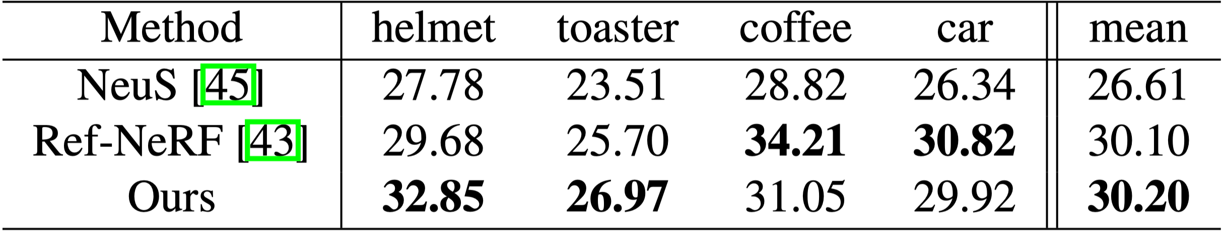
在重建任務的渲染品質比較,本篇方法也與 Ref-NeRF 有可比性。
本篇僅採樣 1024 條射線,而非 Ref-NeRF 使用的 4096 × 4。
Ablation Study#
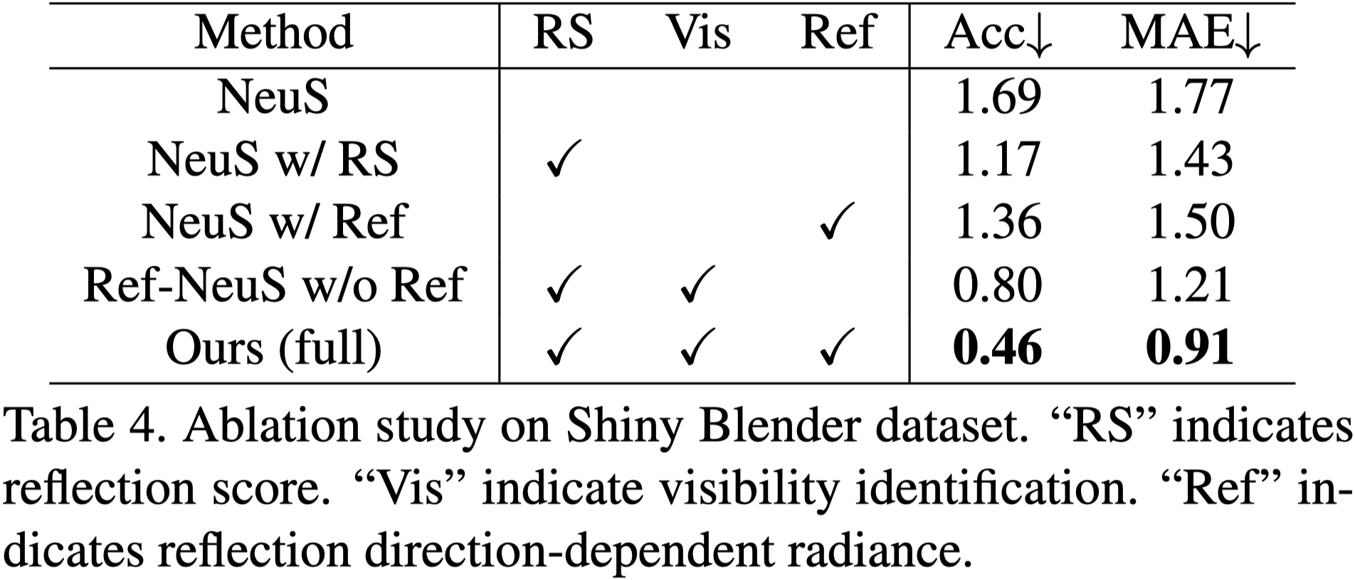
- “NeuS w/ RS”: 使⽤反射分數作為變異數仍然有利於改進幾何形狀。
- 使用反射方向估計 radiance 有效提升效果。
Conclusion#
Limitation
- 計算反射分數會增加計算成本。
- 如果不論物體材質為何,都以反射方向建構輻射場,在某些情況可能導致偽影。
透過引⼊ reflection-aware photometric loss 解決反射導致的多視圖不一致性。
- 通過使用高斯分佈模型降低反射像素的重要性。
- 採用 reflection direction-dependent radiance 進一步改善場景幾何(包括幾何形狀與表面法線)。