
本篇筆記整理自 ICCV 2023 論文《NSF: Neural Surface Fields for Human Modeling from Monocular Depth Scene Reconstruction》。該論文提出一種只需單目深度序列即可學習細緻且可動畫的人體模型的方法,突破了以往 3D 人體重建對高階感測設備與複雜預處理的依賴。核心貢獻為引入 Neural Surface Fields (NSF),在 canonical space 上定義連續的神經場,能高效融合不同姿勢與服裝幾何,實現任意解析度的網格重建,且無需重新訓練。實驗證明 NSF 相較於過往方法有更高效率與更佳的幾何、紋理還原能力,支援快速 few-shot 新人物訓練與高質感動畫生成,並能直接進行紋理轉換。
- Link: https://arxiv.org/abs/2308.14847
- Conference: ICCV 2023
Introduction#
- Purpose
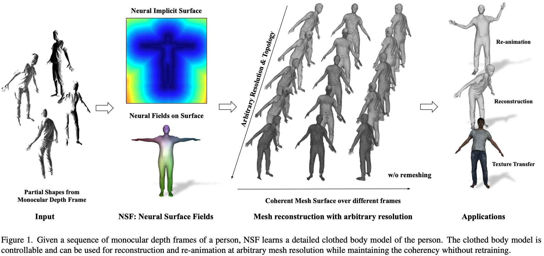
- 僅從單目深度,學習一個靈活且可以跨不同 frames 的穿著衣服的身體模型。
- Previous Works and Challenges
- 4D input
- 需要專門技術、預處理,難以應用。
- 使用消費級的單目深度捕捉設備雖然較為容易獲取,但會有額外的感測器雜訊。
- 使用參數模型作為先驗
- SMPL
- 限制模型的表示能力,例如只能表示緊身服裝。
- 有些方法透過預測 SMPL 頂點上的位移來對人體建模,雖然他們能夠重建連貫的網格,但受到 SMPL template 的解析度和拓樸的限制。
- Point Cloud
- 實際應用需要 3D 網格,因此重建表面時開銷較大。
- 從每幀影像提取表面會增加計算成本,也會導致三角測量不一致。
- SMPL
- 4D input
- Contribution
- 提出 NSF (Neural Surface Fields)
- 一個在 canonical space 的表面上定義的連續 neural field。
- NSF 緊湊、高效,並且無需重新訓練就可以離散化成任意解析度的網格。
- 能保持不同姿勢的一致性。
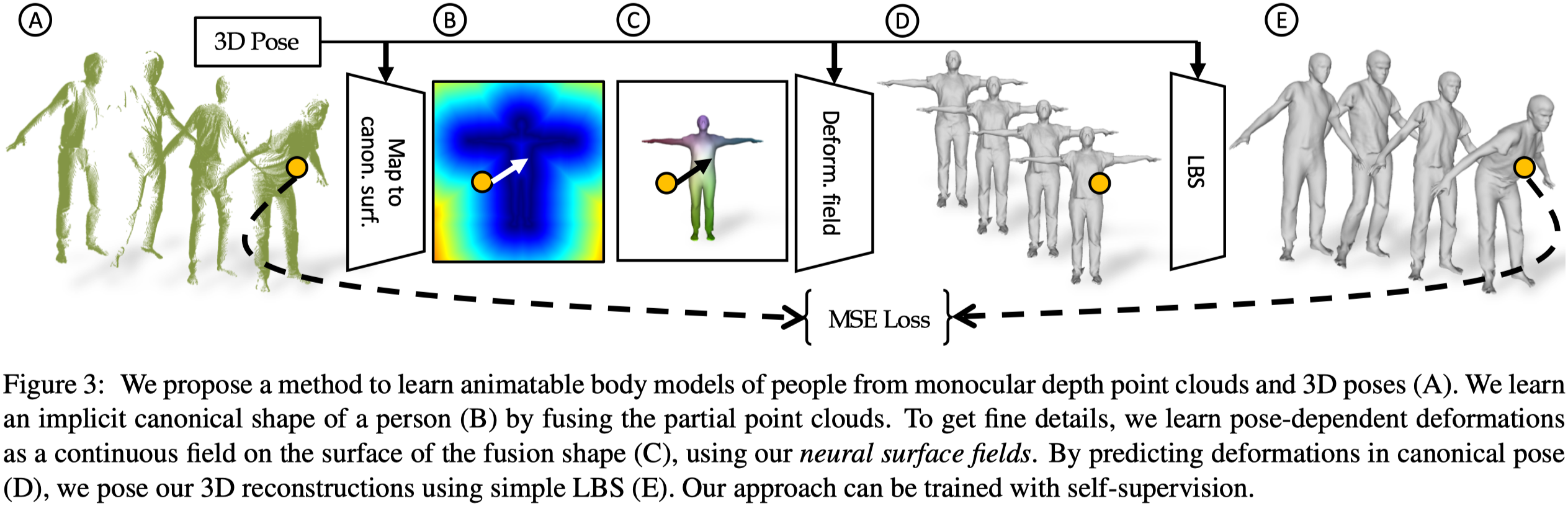
- 提出一種從單目深度序列學習可動畫人體的方法
- NSF 可以從單目深度影格中恢復詳細的形狀資訊。
- 可以處理不同服裝的幾何形狀與紋理。
- 提出 NSF (Neural Surface Fields)
Methods#
NSF: Neural Surface Fields#
Neural Fields#
所謂的 neural field 是由神經網路參數化的 field,表示如 Eq. \eqref{eq:1}:
$$ \begin{equation} f_\phi = \mathbb{R}^m \rightarrow \mathbb{R}^n, \tag{1} \label{eq:1} \end{equation} $$定義在歐式空間中的 neural field 廣泛被使用於表示各種幾何。
Neural Surface Fields#
由於空間中大部分的區域不會被查詢,導致計算和記憶體資源的浪費,因此作者僅在 2D 表面 $\mathcal{S}^2$ 上定義 field:
$$ \begin{equation} f_{\phi} : \mathcal{S}^2 \subset \mathbb{R}^3 \to \mathbb{R}^n. \tag{2} \end{equation} $$NSF for Human Modelling#
Overview#
- Input
- 單目深度點雲序列,$\mathcal{X}^s = \{ \mathbf{X}^s_1, \ldots, \mathbf{X}^s_{T_s} \}$。
- 相對應的 3D poses $\theta$。
- Output
- Subject-specific body models $\mathcal{M} = \{ M^1, \ldots, M^N \}$。每個 model 可以從 canonical space 中轉換而來。
A. 首先使用 inverse LBS 將輸入 point clouds 移除 pose。實際上就是將 input point clouds 轉換至 canonical space 中。
B. 將他們 fuse,以學習一個隱式的 (SDF) canonical shape $\mathcal{B}^s$。本篇的 canonical space 是連續的。
C. 訓練 NSF,用以預測連續的 canonical surface 上每個點的 pose-dependent deformation。
D. 為人物特定姿勢重新覆蓋上 cloth deformation。
E. 使用 LBS 重新將姿勢接入 human model。
整個框架會在 input point cloud 與 predicted shape 之間使用 cycle-consistency loss 優化。
Fusion Shape from Monocular Depth#
Canonicalization
Input points 對應的 canonical points $\mathbf{X}^c_t$ 可以通過 iterative root finding (Eq. \eqref{eq:3}) 找到:
$$ \begin{equation} \underset{\mathbf{X}^c_w, w}{\text{arg min}} \sum_{t=1}^{T} \left( \left( \sum_{i=1}^{K} w(\mathbf{X}_t^c)_i \cdot \mathbf{T}_i(\theta_t) \right) \mathbf{X}_t^c - \mathbf{X}_t \right). \tag{3} \label{eq:3} \end{equation} $$符號 描述 $K$ The number of joints. $w(\cdot)$ The skinning weights for joint $i$. $\mathbf{T}_i$ The joint transformation for joint $i$. 除了 iterative root finding,作者同時還利用 FiTE 的 pre-diffused SMPL skinning field 來避免模糊的結果。
通過這樣的方式,我們可以將 input observation $\mathcal{X} = \{ \mathbf{X}_t \}^T_{t=1}$ 轉換至 partial shapes $\mathcal{X}^c = \{ \mathbf{X}^c_t \}^T_{t=1}$。
Implicit Fusion Shape
轉換後的 point cloud $\mathbf{X}^c_t$ 仍然包含特定 subject 的 non-rigid deformation,為此作者需要進一步的將單一姿勢的影響消除。
作者的做法是透過在 canonical space 中學習一個隱式的表面來融合每個主體的 point cloud。
具體做法是,遵循 Deepsdf 的作法將 canonical shape 表示成隱式的 SDF (Signed Distance Function)。通過一個網路 $f^{\text{shape}}(\cdot | \phi^{\text{shape}})$ ,以 subject specific latent code $\mathbf{h}^s \in \mathbb{R}^{256}$ 與 query point $\mathbf{x} \in \mathbb{R}^e$ 作為輸入並輸出 SDF 值。
$$ \begin{equation*} \text{SDF}: f^{\text{shape}}(\mathbf{x}^c_i, \mathbf{h}^s | \phi^{\text{shape}}) \end{equation*} $$Subject-specific latent codes $\mathcal{H} = \{ \mathbf{h}^s \}^N_{s=1}$ 與 decoder parameters $\phi^{\text{shape}}$ 是通過 self-supervised 優化,如 Eq. \eqref{eq:4}, Eq. \eqref{eq:5} 所示:
$$ \begin{equation} E^{\text{shape}}(\phi^{\text{shape}}, \mathcal{H}) = E_{\text{geo}} + \lambda_1 E_{\text{eik}} \tag{4} \label{eq:4} \end{equation} $$$$ \begin{align*} E_{\text{geo}}(\phi^{\text{shape}}, \mathcal{H}) = \sum_{s=1}^{N} \sum_{t=1}^{T^s} \sum_{i=1}^{L_{s,t}} ( \left| f^{\text{shape}}(\mathbf{x}^c_i, \mathbf{h}^s | \phi^{\text{shape}}) \right| + \\ \lambda_3 \left| \nabla_{\mathbf{x}} f^{\text{shape}}(\mathbf{x}^c_i, \mathbf{h}^s | \phi^{\text{shape}}) - \mathbf{n}^c_{i} \right|_2 ), \tag{5} \label{eq:5} \end{align*} $$符號 描述 $\mathbf{n}_i$ The normal along with the point $\mathbf{x}_i$ in observation space which is computed using Kinectfusion. $\mathbf{n}^c_t$ The normal obtained by canonicalising $\mathbf{n}_i$. $\nabla_{\mathbf{x}}$ The spatial derivative. $E_\text{eik}(\cdot)$ 強制 canonical surface 上的 SDF 預測值應該為 0,並且他的導數(法線方向)應該與 canonicalised normal 相匹配:
$$ \begin{equation} E_{\text{eik}}(\phi^{\text{shape}}, \mathcal{H}) = \sum_{s=1}^{N} \sum_{t=1}^{T^s} \sum_{i=1}^{L_{s,t}} \left( \left| \nabla_{\mathbf{x}} f^{\text{shape}}(\mathbf{x}^c_i, \mathbf{h}^s | \phi^{\text{shape}}) \right|_2 - 1 \right)^2. \tag{6} \end{equation} $$小結
Fusion shape 允許我們對每個主體,將所有的 partial canonical frames 融合成單一且連續的 shape。
之前的方法(Intrinsic neural fields)利用 Laplace-Beltrami Operator 在表面上的特徵函數來定義 neural field,因此僅適用於幾何的特定離散化。
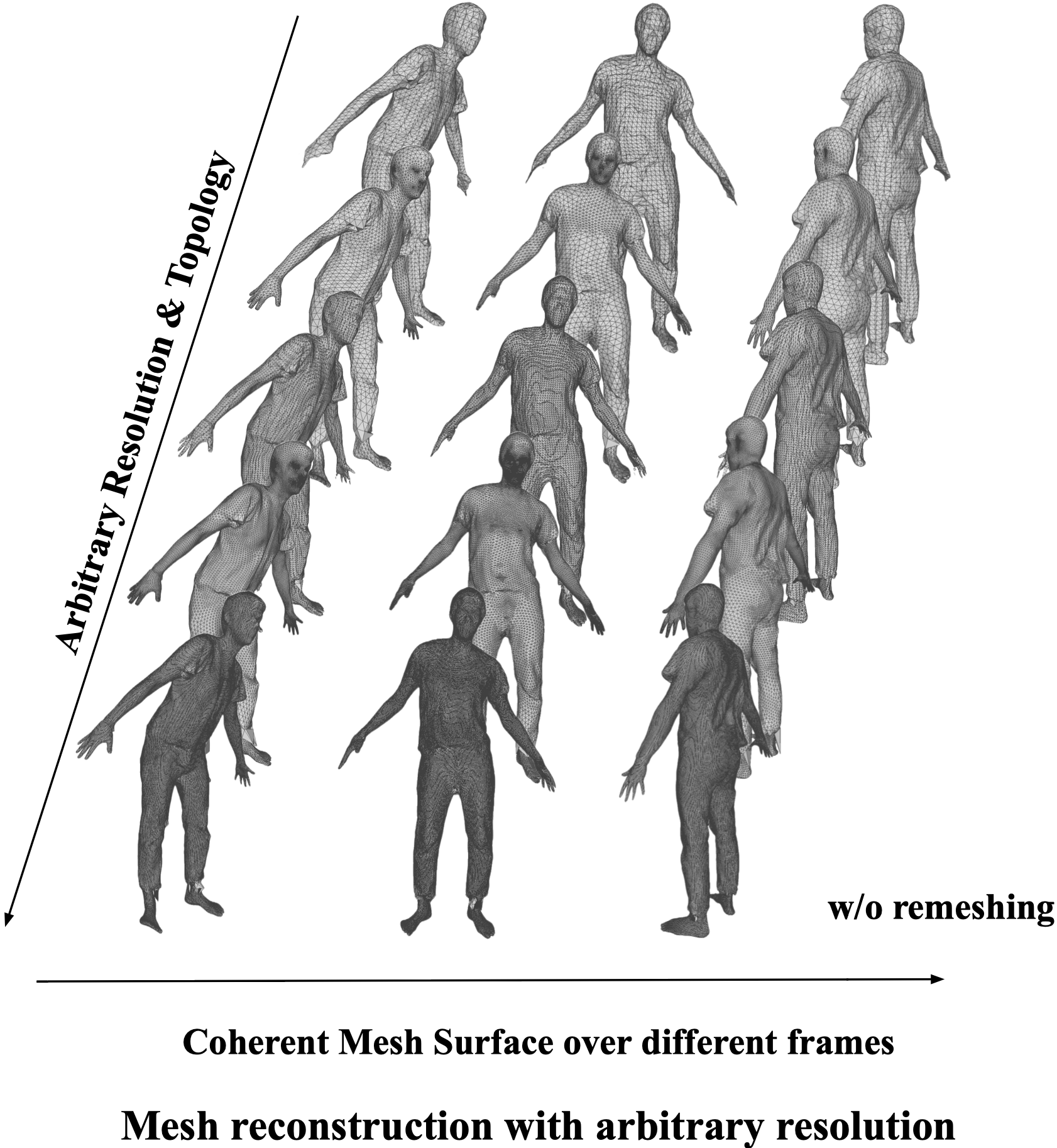
而 NSF 更加通用,並可以產生物體的連續場。他能將網格表面的連貫性與連接性結合。
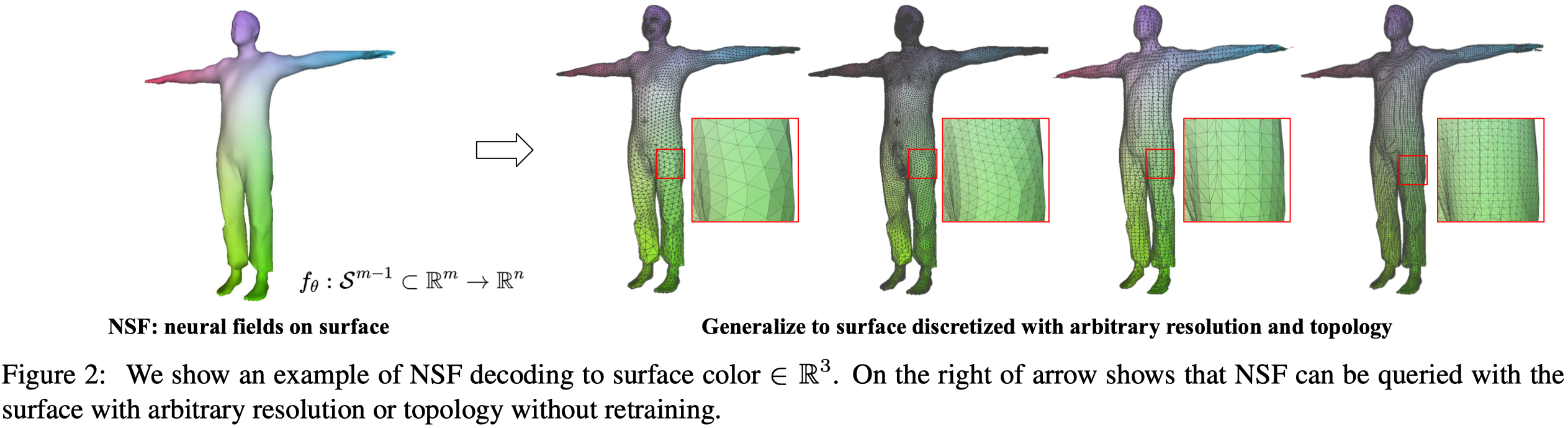
Fig.2: 在箭頭右側可見, NSF 無需重新訓練即可使用任意解析度或拓樸查詢。
Canonical shape 的 subject-specific geometry 可以使用對應的 latent codes 編碼而成。
這樣的方法可以讓 decoder 可以自由地學習跨主體的共同資訊。
NSF for Pose-Dependent Deformation#
Neural Surface Deformation Field
前面的方法通過融合 input observation 來學習 pose-independent fusion shape。但為了忠實呈現人體詳細的形狀,作者需要構建細緻的 pose-dependent deformations。
利用 NSF,作者在 fusion shape surface $\mathcal{B}^s$ 上定義了一個 deformation field:
$$ \begin{equation} f_{\phi} : \mathcal{S}^2 \subset \mathbb{R}^3 \to \mathbb{R}^3, \tag{7} \end{equation} $$主體的 deformed points 可以通過 Eq. \eqref{eq:8} 得到:
$$ \begin{equation} \mathbf{X}^p = \mathbf{X}^c + f^{\text{pose}}(\mathbf{F}^s(\mathbf{X}^c), \theta | \phi^{\text{pose}}), \tag{8} \label{eq:8} \end{equation} $$符號 描述 $\mathbf{F}^s(\cdot)$ The latent feature queried at point $\mathbf{x}^c$ for subject. $\theta$ The pose feature. 有兩個挑戰:
- 如何學習表面上的 feature $\mathbf{F}^s(\cdot)$?
- 如何處理不在表面上的 query points?
Feature Learning On Surface
- 透過 Marching Cubes [38] 離散化隱式 fusion shape 來提取顯式表面。
- 使用在表面上定義 $5000 \sim 7000$ 個頂點來作為特徵的基礎位置。
- 使用 auto-decoder 獲取頂點特徵。
- 任意表面點的特徵可以通過將鄰近三個頂點特徵作重心插值獲得。
這樣的方法仍然保有 3D 的空間排列。
此外也更有記憶體效率,比如一般使用解析度為 128 的 volumetric latent features ,模型需要學習 $128^3$ 個特徵;而本篇基於表面的方法僅需要學習約 7000 個特徵。
Projecting Off-surface Points Onto Surface
作者使用先前預訓練的 auto-decoder 來獲得 canonical point 對應的 SDF。SDF 的梯度提供我們垂直於表面的法線方向。
接著就可以通過 Eq. \eqref{eq:9} 找到 $\mathbf{x}^c$ 所對應的表面點 $\mathbf{x}^{cc}$:
$$ \begin{equation} \mathbf{x}^{cc} = \mathbf{x}^c + f^{\text{shape}}(\mathbf{x}^c, \mathbf{h}^s | \phi^{\text{shape}}) \nabla_{\mathbf{x}_c} f^{\text{shape}}(\mathbf{x}^c, \mathbf{h}^s | \phi^{\text{shape}}). \tag{9} \label{eq:9} \end{equation} $$通過 surface projection ,就可以讓這些不在表面上的點,根據對應的投影表面點做變形。
Self-supervised Cycle Consistency#
Reposing via Skinnning
通過 LBS 將 canonical pose 賦予姿勢:
$$ \begin{equation} \mathbf{X}^{pp} = \left( \sum_{i=1}^{K} w_i(\mathbf{X}^p) \mathbf{T}_i(\theta) \right) \mathbf{X}^p, \tag{10} \end{equation} $$符號 描述 $\mathbf{X}^p$ The NSF predicted pose-dependent canonical points. $\mathbf{X}^{pp}$ The reposed pose-dependent points. $\mathbf{X}^{pp}$ 可以看作 input observation $\mathbf{X}_t$ 的重建。
Self-supervised Learning
為了確保 posed reconstruction 與 input point cloud 匹配,作者使用 Eq. \eqref{eq:11}, Eq. \eqref{eq:12} 來做 self-supervised。
$$ \begin{align*} E^{\text{pose}}(\phi^{\text{pose}}, \mathcal{F}) = \sum_{s=1}^{N} \sum_{t=1}^{T^s} \sum_{i=1}^{L_{s,t}} ( \left| \mathbf{x}_i - \mathbf{x}_i^{pp} \right|_2 + \left| \mathbf{n}_i - \mathbf{n}_i^{pp} \right|_2 \\ + d^{\text{CD}}(\mathbf{x}_i, \mathbf{x}_i^{pp}) + E^{\text{reg}}_{\text{pose}}), \tag{11} \label{eq:11} \end{align*} $$$$ \begin{equation} E_{\text{reg}}^{\text{pose}} = \left| \mathbf{x}_i^p - \mathbf{x}_i^c \right|_2 + \left| F^s(\mathbf{x}_i^c) \right|_2 + EDR(\mathbf{x}_i^c), \tag{12} \label{eq:12} \end{equation} $$$$ \begin{equation*} EDR(\mathbf{x}_i^c) = \left| F^s(\mathbf{x}_i^c) - F^s(\mathbf{x}_i^c + \omega) \right|_2 \end{equation*} $$符號 描述 $\omega$ The random small scalar. $d^{\text{CD}}(\cdot, \cdot)$ The uni-directional Chamfer distance. $\mathbf{x}_i^{pp}$ The predicted skinned points. Eq. \eqref{eq:11} 強制預測的 skinned points 與對應的法向量跟輸入的 posed points 與法向量相匹配。
The regularisation term $E_{\text{reg}}^{\text{pose}}$ :
- Deformation field 上的 L2 regulariser。
- EDR term 強制 feature space 上的空間平滑性。
Inference and Surface Extraction#
- 推理階段
- 預測 base fusion shape 頂點的 pose-dependent deformation。
- 通過 LBS 獲得 pose space 的位置。
- 由於 NSF 是連續表面,因此作者在 fusion shape 上使用 original edge connectivity,並對頂點賦予姿勢來獲得 posed mesh。
- 重建
- Freeze the deformation function。
- 使用 Laplacian smoothness loss 最小化 input partial shape 與 reconstructed mesh 之間的 single-directional Chamfer distance。
Experiments#
Experimental Setting#
Datasets
- BuFF
- CAPE
- DSFN(real data)
資料集中有包含 Kinect camera 資料(深度相機)
Metrics
- Chamfer distance (in cm):量測點雲的誤差。
- Normal correctness
- IoU:量測 ground-truth mesh 與重建結果的誤差。
Baselines
- PINA (與本篇有相似的問題設定)
- DSFN:從單目 RBG-D 影片中學習 SMPL-based 3D avatars
PINA 與 DSFN沒有發布程式碼,因此作者使用 BuFF 資料集驗證本篇方法,並使用他們論文中展示的數值比較。
- POP
- MetaAvatar
- NPMs
- 本篇的 baseline:使用 naked SMPL shape 與 learned fusion shape (w/o NSF).
這些基線強調了在 NSF 中學習姿勢相關變形的重要性。
Reconstruction Comparison with Baselines#
⽬標是恢復完整穿著衣服的⾝體模型。
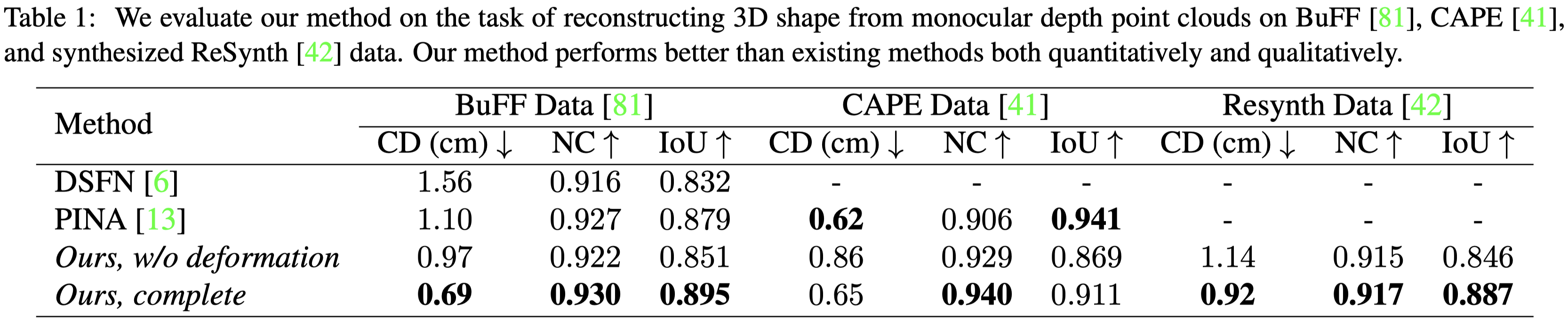
競爭⽅法 [6,13] 需為每個受試者訓練⼀個神經網絡,我們的⽅法是跨多個受試者進⾏訓練的,可以⽤更少的計算資源產⽣更可靠的重建。
在 DuFF 資料及上比較 DSFN 與 PINA。
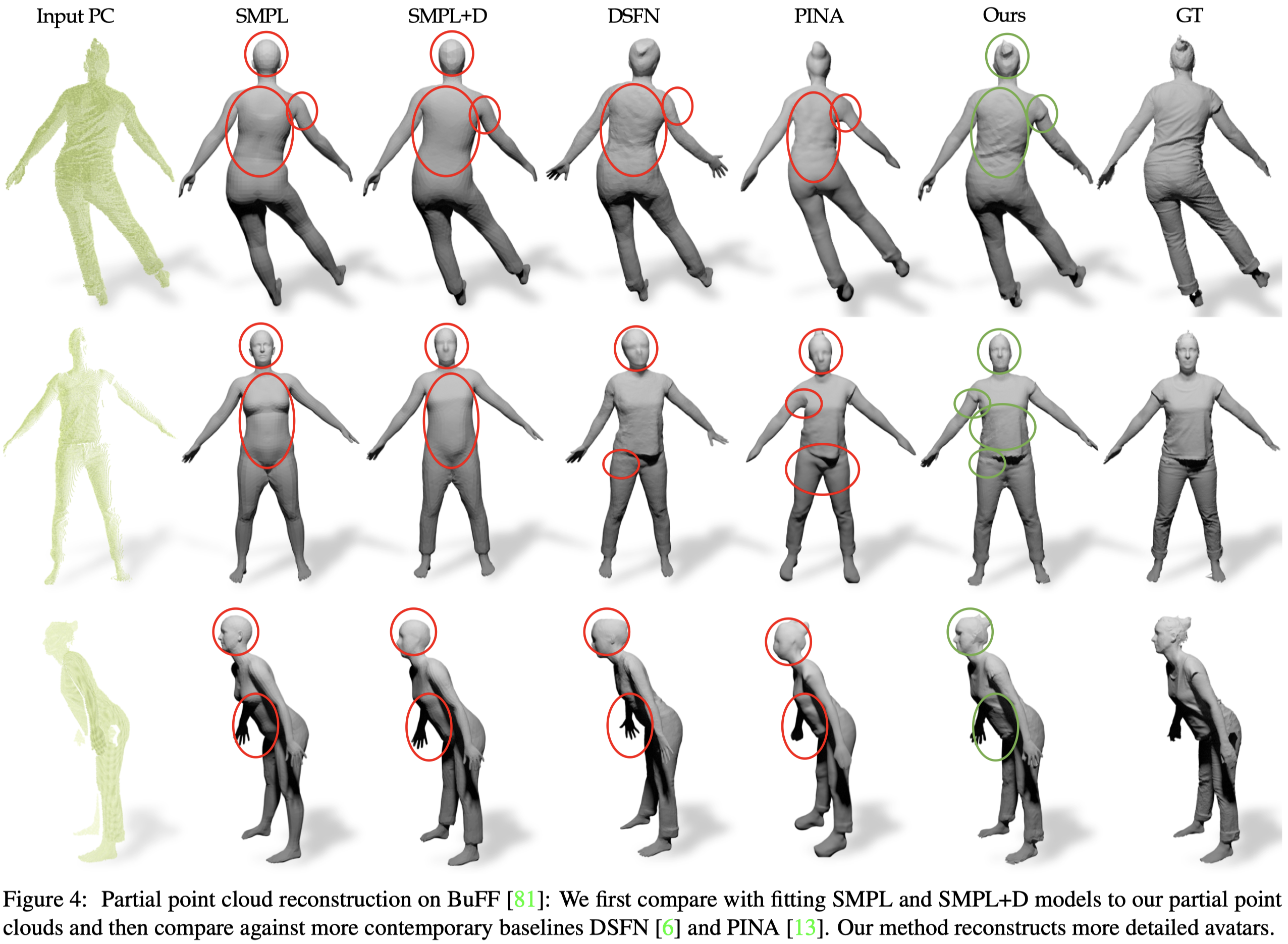
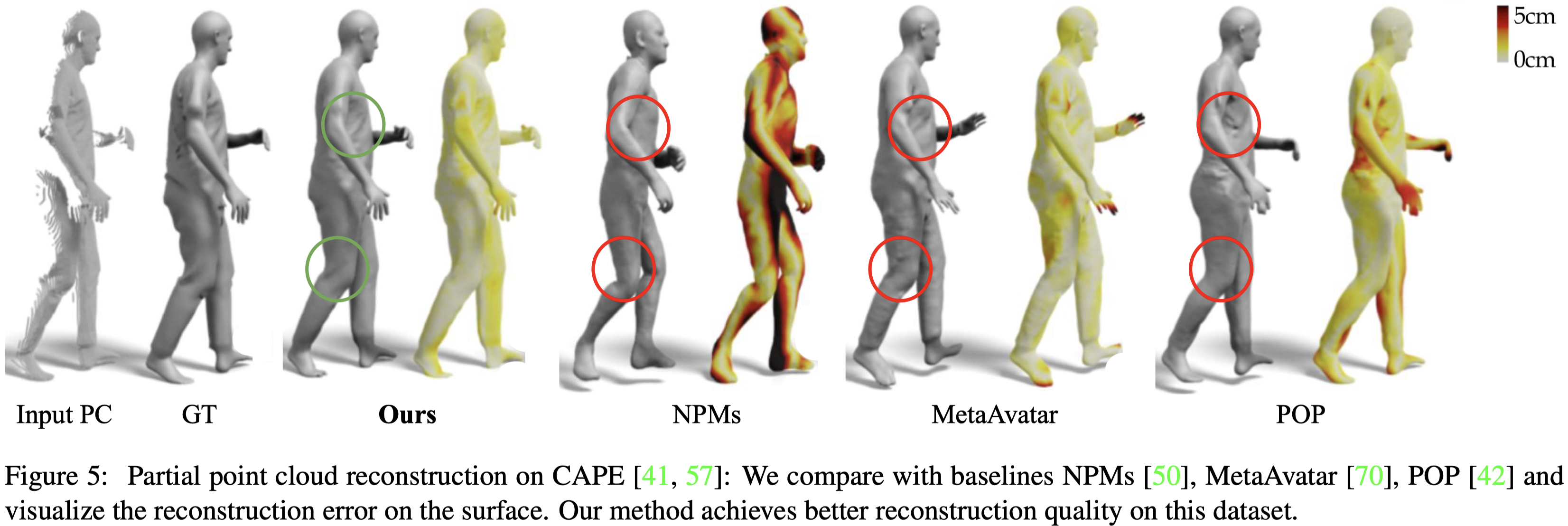
在 CAPE 資料及上評估其他的方法。
可以以任意解析度重建⼀序列的連貫網格,⽽無需重新訓練。
這是其他的 baseline 無法做到的。
Efficiency of Neural Surface Field#
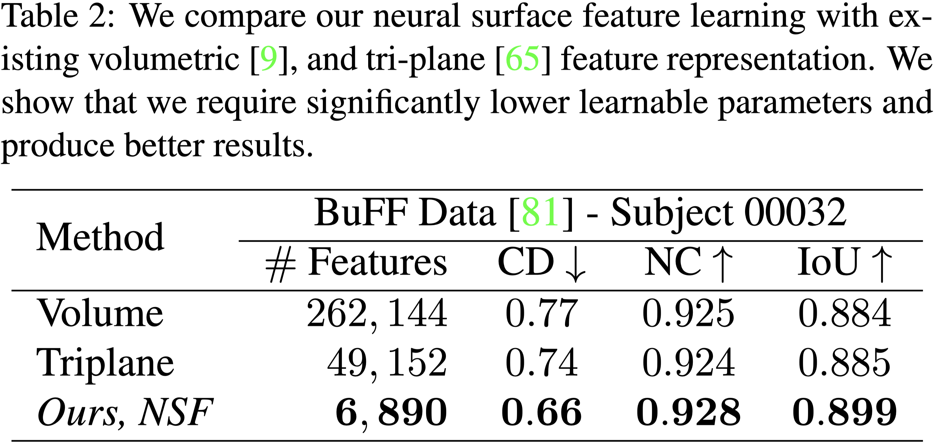
- 在這個實驗中,作者使用相同的網路與資料設計三種變體:
- Volumetric
- Tri-plane
- NSF
- 本篇的方法可以取得做好的效果。
- 與其他兩種方法相比,NSF 的學習特徵少了約 10~100 倍。
- 由於不需要 per-frame surface extraction,因此 NSF 的推理速度也比其他方法快 40~180 倍。
Importance of Feature Fecoupling: Learning a New Avatar with 10 images in under 10 mins#
本篇的方法能將泛化神經網路與特定主體的特徵解耦,因此可以使用少量的資料,快速學習新的特定主體的特徵。(10 張深度影像,訓練 10 分鐘)
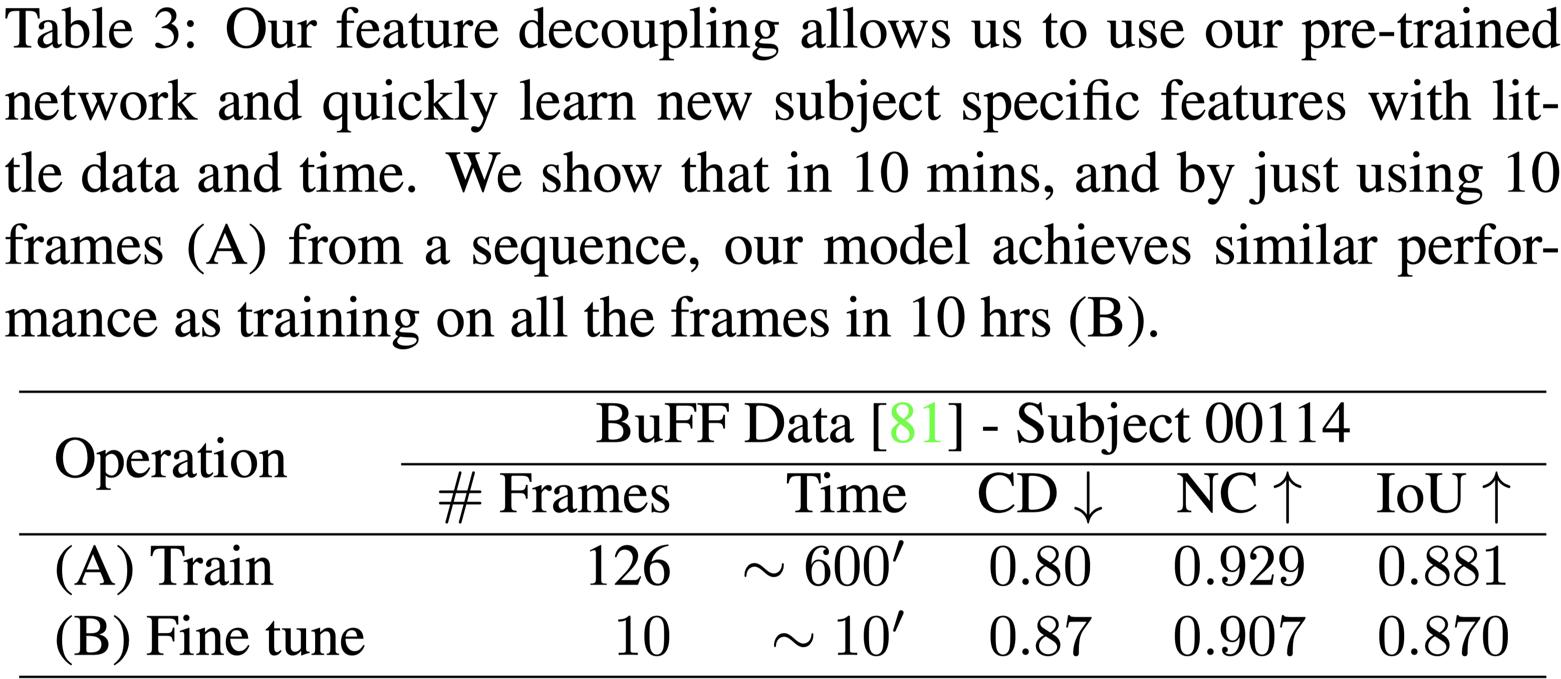
在 Tab.3 中呈現,訓練完整的網路需要約 10 小時。
當我們只使用三個主體做訓練,並使用第四個主體的 10 個隨機幀做評估,仍然可以獲得與完整訓練相近的效果。
而其他的方法並沒有這種能力。
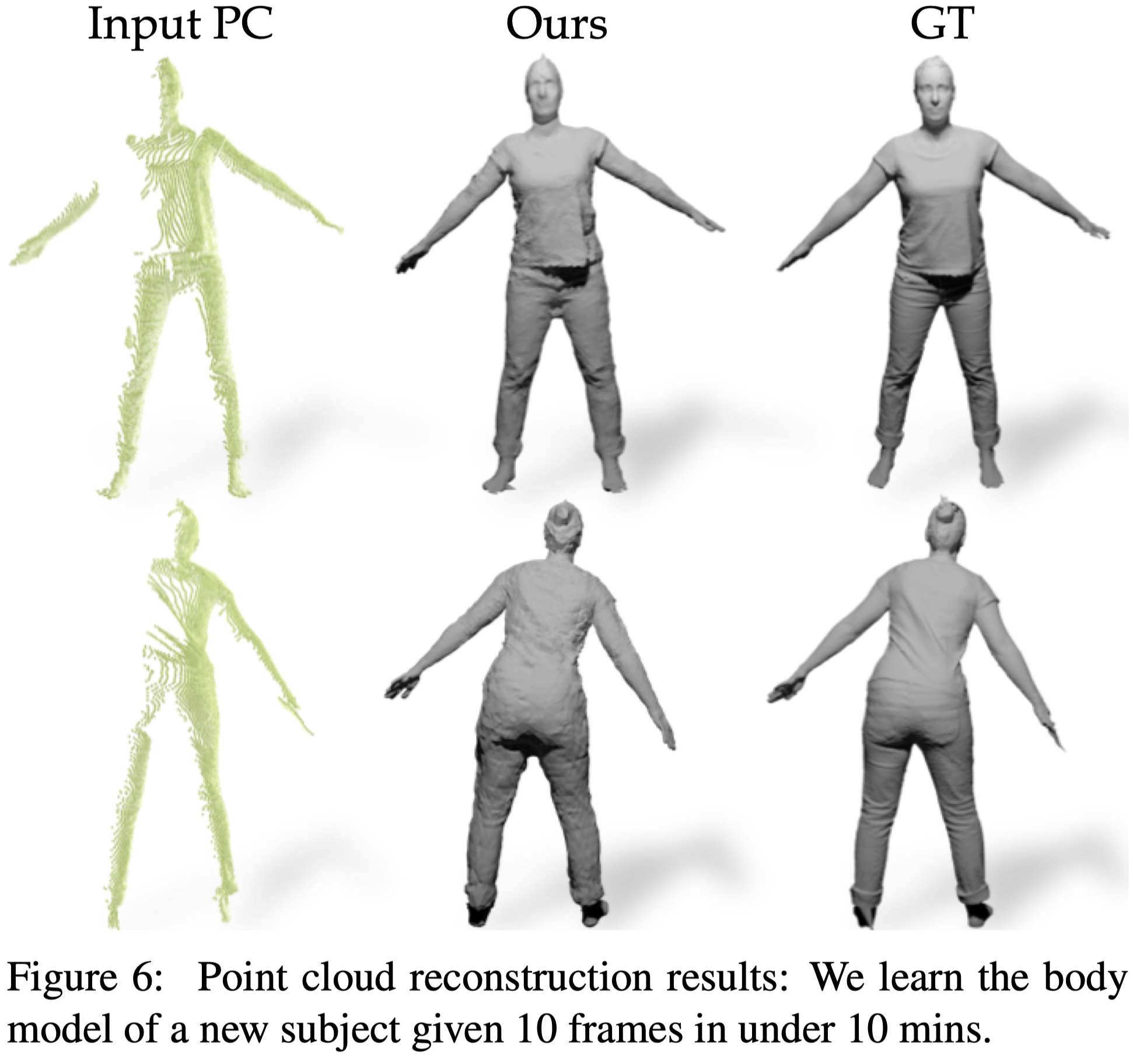
Fig.6 展示了重建結果。
Animating Learnt Avatars#
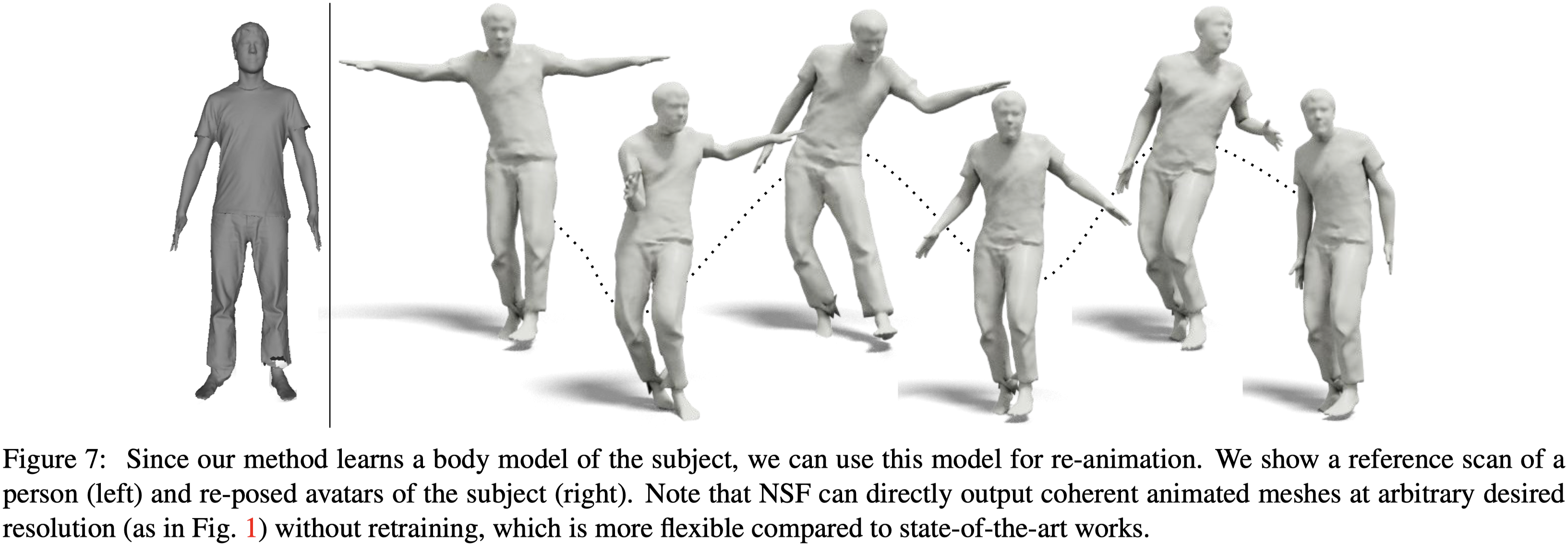
作者在 BuFF 資料集上訓練模型,然後使用 AIST 資料集的姿勢做人體動畫。
Results on Real Data#
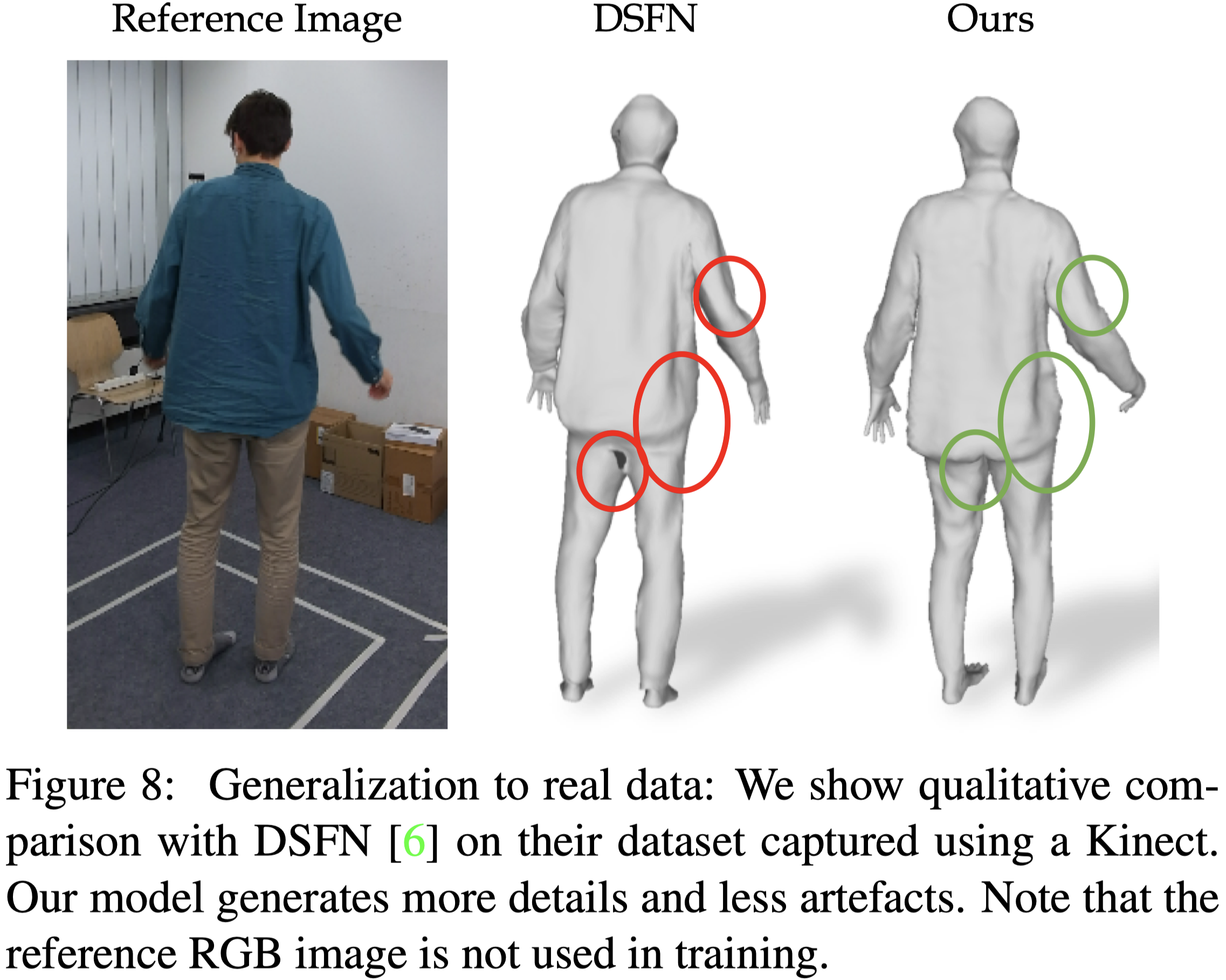
本篇的方法在真實資料集也比以往的方法有更好的表面結構。
Learning Textured Avatars#
本篇的方法在 input pose space 與 fusion shape 有明確的對應關係,因此能夠直接將紋理從 input point cloud 轉換至 canonical pose 上。
Baseline 的方法並沒有這樣的能力。
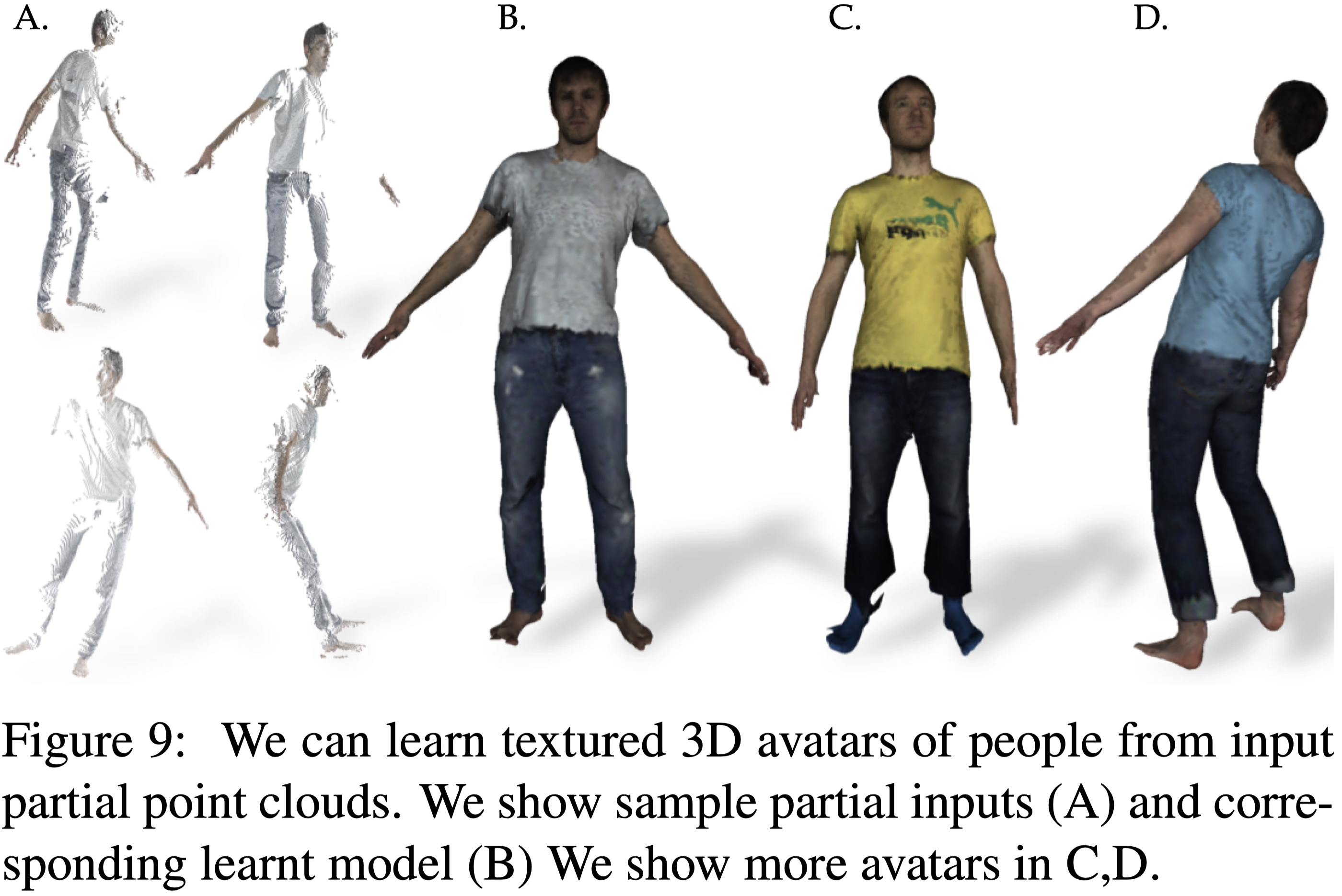
Fig.9 展示本篇 textured 3D avatar 的範例。
Conclusion#
- 提出了 Neural Surface Fields (NSF):一種用於建模穿著服裝的人體的高效、細緻的 manifold-based continuous fields。
- 不需重新訓練,即能夠重建任意解析度的網格,同時保持網格的連貫性。
- 消除了昂貴的 per-frame surface extraction,推理時間比 baseline 快約 40~180 倍。
- 結構緊湊,並保留了 underlying manifold 的 3D 結構。
- 支援如 texture transfer 和 fine-tuning 以適應新主體等應用。