
本篇筆記整理了 NeuS (NeurIPS 2021) 的研究內容。該論文致力於從多視角影像(multi-view images)中實現高品質的 3D 表面重建,旨在結合隱式表面表示(implicit surface representation)和體積渲染(volume rendering)的優點,同時克服先前方法(如 IDR 和 NeRF)各自的局限性。筆記內容涵蓋了其核心方法:將 3D 表面表示為神經符號距離函數(Neural Signed Distance Function, SDF)的零水平集(zero-level set),並提出一種新穎的體積渲染方案來訓練此 SDF 網路。此方案的關鍵在於設計了一個基於 SDF 導數(S-density)的權重函數(weight function)和對應的不透明度密度(opaque density),使其既能無偏差地(unbiased)定位表面,又能處理遮擋(occlusion-aware)。此外,筆記也記錄了其訓練細節,包括損失函數(包含顏色損失、Eikonal 正規化和可選的遮罩損失)以及層級採樣(hierarchical sampling)策略,最終目標是重建出高保真度的物體表面。
- Link: https://arxiv.org/abs/2106.10689
- Conference: NeurIPS 2021 {: .prompt-info }
Introduction#
Purpose
- 高品質表面重建。
Previous Works and Challenges
- IBR
- 其使用的 surface rendering 會在深度發生突變時,陷入局部最小值,如 Fig.1 (a)。
- 需要物體的 masks 做監督,來約束有效表面。
- NeRF
- 優點:volume rendering 可以處理深度突變。
- 缺點:
- 只學習 volume density field 無法提取出高品質的表面。
- 儘管可以還原突然的深度變化,但在某些平面區域中包含明顯雜訊。
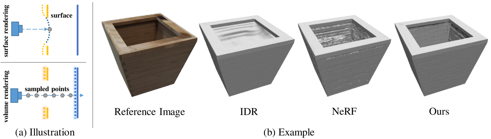
Figure 1: (a) Illustration of the surface rendering and volume rendering. (b) A toy example of bamboo planter, where there are occlusions on the top of the planter. Compared to the state-of-the-art methods, our approach can handle the occlusions and achieve better reconstruction quality. - IBR
Contribution
- 以 volume rendering 技術來學習隱式 SDF 表示。
- 由於直接使用標準 volume rendering 到與 SDF 相關的密度會導致重建表面的偏差。因此作者提出了一種新的 volume rendering 方案。
- 優於 SOTA 的神經場景表示方法 (IDR, NeRF)。
Methods#
目標是重建物體表面,此表面由神經隱式 SDF 的 zero-level 表示。
為了學習神經網路的權重,作者開發了一種新的 volume rendering 方法。
Overview#
Rendering Procedure#
Scene Representation#
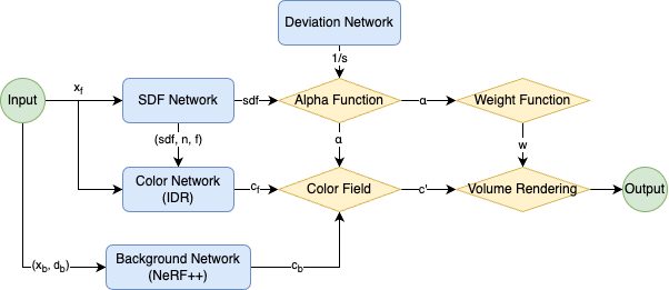
場景的重建表示成下面兩個 function:
$$ \begin{align*} f&: \mathbb{R}^{3} \rightarrow \mathbb{R} \\ c&: \mathbb{R}^{3} \times \mathbb{S}^{2} \rightarrow \mathbb{R}^{3} \end{align*} $$$f$ 用於將空間座標 ($\mathbb{R}^{3}$) 映射到其到物體的 signed distance。
$c$ 用於根據點 ($\mathbb{R}^3$) 與 viewing direction ($\mathbb{S}^{2}$) 來編碼顏色。
物體的表面 $\mathcal{S}$ 可以寫成 Eq. \eqref{eq:1}:
$$ \begin{equation} \mathcal{S} = \{ \mathbf{x} \in \mathbb{R}^{3} | f(\mathbf{x}) = 0 \}. \tag{1} \label{eq:1} \end{equation} $$為了應用 volume rendering 來訓練 SDF network,作者引入 probability density function $\phi_{s}(f(\mathbf{x}))$,稱為 S-density。
$$ \begin{equation*} \phi_{s}(x) = \frac{se^{-sx}}{(1+e^{-sx})^{2}} \end{equation*} $$其中 $\phi_{s}(x) = \frac{se^{-sx}}{(1+e^{-sx})^{2}}$ 是 SIgmoid function $\Phi_{s}(s) = (1+e^{-sx})^{-1}$ 的導數,即 $\phi_{s}(x) = \Phi_{s}'(x)$。
$\phi_{s}(x)$ 的標準差為 $1/s$,也是 trainable parameter,訓練後趨近於 0。
NeuS 的主要思想是借助 S-density field,使用 volume rendering 來訓練網路。基於此監督,SDF 的 zero-level 集合即為重建表面。
Rendering#
假設從該像素發出的光線表示為 $\{ \mathbf{p}(t) = \mathbf{o} + t \mathbf{v} | t \geq 0 \}$ ,$\mathbf{o}$ 是相機原點,$\mathbf{v}$ 是 viewing direction。沿著射線的累積顏色可以表示成 Eq. \eqref{eq:2}:
$$ \begin{align*} C(\mathbf{o}, \mathbf{v}) = \int_{0}^{+\infty} w(t)c(\mathbf{p}(t), \mathbf{v})dt, \tag{2} \label{eq:2} \end{align*} $$| 符號 | 描述 |
|---|---|
| $\mathbf{p}(t)$ | The sampled point. |
| $\mathbf{o}$ | The camera position. |
| $\mathbf{v}$ | The viewing direction. |
| $C(\mathbf{o}, \mathbf{v})$ | The output color for this pixel. |
| $w(t)$ | The weight of the point. |
| $c(\mathbf{p}(t), \mathbf{v})$ | The color at the point. |
Requirements on weight function#
- Unbiased
- 規則:在表面交點獲得局部最大值。
- 確保相機光線與 SDF 的 zero-level set 的相交像素顏色貢獻度最大。
- Occlusion-aware
- 規則:當給定任意兩個深度值 $t_0$ 和 $t_1$,若滿足 $f(t_0) = f(t_1)$ 、 $w(t_0) > 0$ 、 $w(t_1) > 0$ 以及 $t_0 < t_1$,則 $w(t_0) > w(t_1)$。也就是說,當兩個點具有相同的 SDF 值,更靠近視點的點具有更大的貢獻度。
- 確保當光線循序通過多個表面時,正確使用最近相機的表面顏色來計算輸出顏色。
Naive Solution#
為了使權重函數能夠感知遮擋,一個簡單的解決方案是使用標準的 volume rendering:
$$ \begin{align*} w(t) = T(t)\sigma(t), \tag{3} \end{align*} $$$$ \begin{equation*} T(t) = \exp (\int^{t}_{0} \sigma(u)du) \end{equation*} $$| 符號 | 描述 |
|---|---|
| $\sigma(t)$ | The volume density in classical volume rendering. |
| $T(t)$ | The accumulated transmittance along the ray. |
這樣的計算方式是有 bias 的,如 Fig.2 (a) 所示,weight function 在到達表面之前就已達到局部最大值。
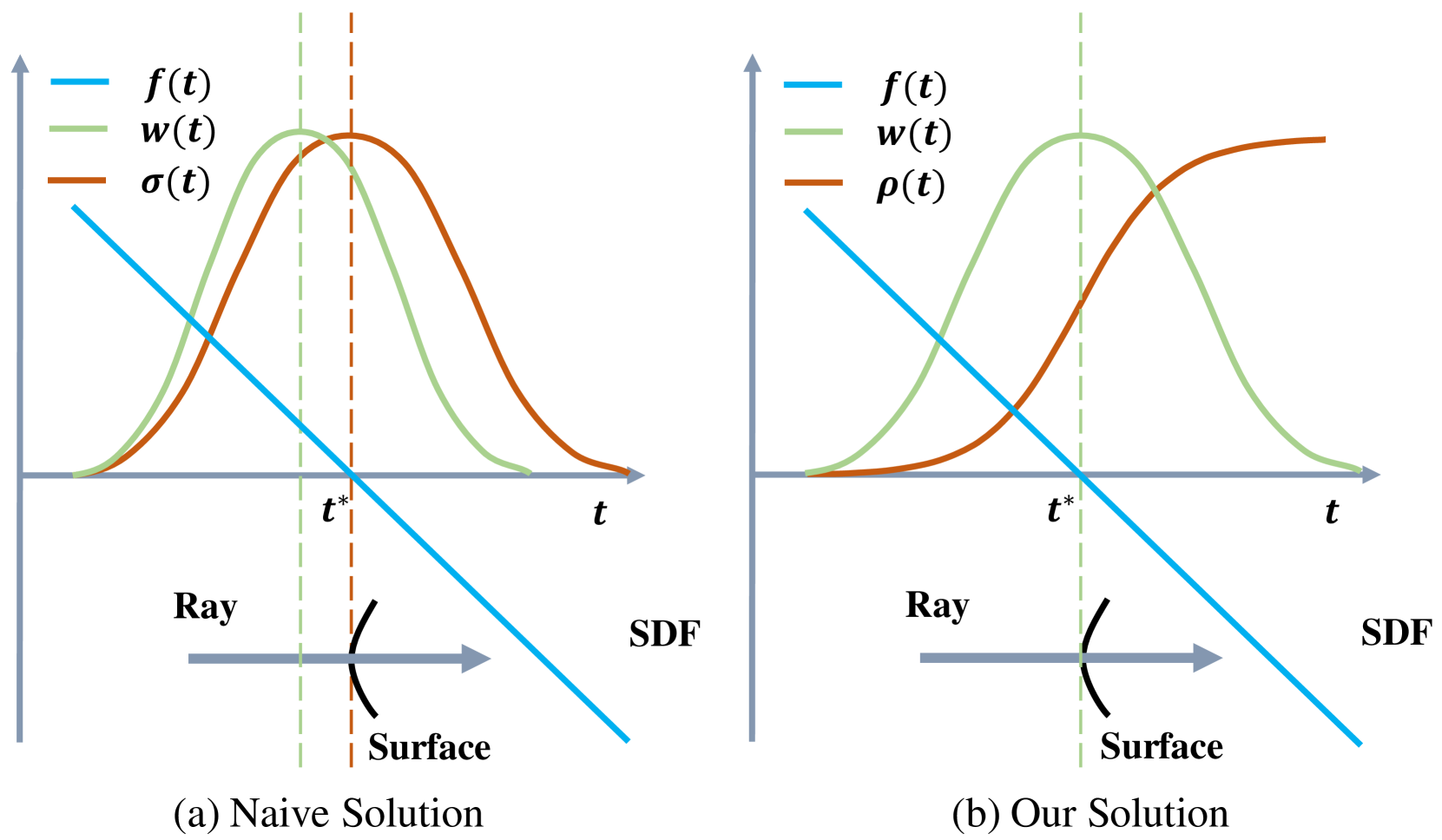
Our Solution#
為了解決上述問題,首先需要使用一個 unbiased weight function,即直接使用 normalized S-density 作為權重:
$$ \begin{align*} w(t) = \frac{\phi_s(f(\mathbf{p}(t)))}{\int_{0}^{+\infty} \phi_s(f(\mathbf{p}(u)))du}. \tag{4} \label{eq:4} \end{align*} $$然而這種 weight function 無法感知遮擋。因此需要遵循標準 volume rendering 框架進行設計。作者首先定義一個不透明密度函數 $\rho(t)$,以替代標準 volume rendering 中的 $\sigma$:
$$ \begin{align*} w(t) = T(t)\rho(t), \text{ where } T(t) = \exp\left(-\int_{0}^{t} \rho(u)du\right). \tag{5} \label{eq:5} \end{align*} $$How We Derive Opaque density $\rho$#
單平面
若考慮只有一個表面相交的情況, Eq. \eqref{eq:4} 確實滿足了上面的要求。
如果只是單一表面,並且其為一平面,可以很容易得到他的 SDF $f(\mathbf{p}(t))$ 是 $-|\cos(\theta)| \cdot (t-t^*)$。其中 $\theta$ 是 viewing direction 與表面法向量的夾角。
由於表面假設為一平面,因此 $| \cos(\theta)|$ 是常數,那 Eq. \eqref{eq:4} 可以通過推導得到 Eq. \eqref{eq:6}:
$$ \begin{equation} \begin{aligned} w(t) &= \lim_{t^* \to +\infty} \frac{\phi_s(f(\mathbf{p}(t)))}{\int_{0}^{+\infty} \phi_s(f(\mathbf{p}(u)))\mathrm{d}u} \\&= \lim_{t^* \to +\infty} \frac{\phi_s(f(\mathbf{p}(t)))}{\int_{0}^{+\infty} \phi_s(-|\cos(\theta)|(u - t^*))\mathrm{d}u} \\&= \lim_{t^* \to +\infty} \frac{\phi_s(f(\mathbf{p}(t)))}{\int_{-t^*}^{+\infty} \phi_s(-|\cos(\theta)|u^*)\mathrm{d}u^*} \\&= \lim_{t^* \to +\infty} \frac{\phi_s(f(\mathbf{p}(t)))}{|\cos(\theta)|^{-1} - \int_{-|\cos(\theta)|t^*}^{+\infty} \phi_s(\hat{u})\mathrm{d}\hat{u}} \\&= |\cos(\theta)|\phi_s(f(\mathbf{p}(t))). \end{aligned} \tag{6} \label{eq:6} \end{equation} $$由於 volume rendering 定義為 $T(t) \rho(t)$,因此可以表示成 Eq. \eqref{eq:7}:
$$ \begin{align*} T(t)\rho(t) = |\cos(\theta)|\phi_s(f(\mathbf{p}(t))). \tag{7} \label{eq:7} \end{align*} $$推導過程:
由於 $T(t) = \exp(-\int^t_0 \rho(u)\mathrm{d}u)$ ,因此:
$$ \begin{equation*} T(t) \rho(t) = - \frac{\mathrm{d}T}{\mathrm{d}t}(t) \end{equation*} $$前面有提到 $|\cos(\theta)|\phi_s(f(\mathbf{p}(t))) = -\frac{\mathrm{d}\Phi_s}{\mathrm{d}t}(f(\mathbf{p}(t)))$ ($\Phi$ 是 Sigmoid function),因此:
$$ \begin{equation*} \frac{\mathrm{d}T}{\mathrm{d}t}(t) = \frac{\mathrm{d}\Phi_s}{\mathrm{d}t}(f(\mathbf{p}(t))) \end{equation*} $$等式兩邊同時積分:
$$ \begin{align*} T(t) = \Phi_s(f(\mathbf{p}(t))). \tag{8} \end{align*} $$取對數,並求導:
$$ \begin{equation} \begin{aligned} \int_{0}^{t} \rho(u) \mathrm{d}u &= - \ln(\Phi_s (f(p(t)))) \\\Rightarrow \rho(t) &= \frac{-\frac{\mathrm{d}\Phi_s}{\mathrm{d}t} (f(p(t)))}{\Phi_s (f(p(t)))}. \end{aligned} \tag{9} \end{equation} $$
這是單平面相交情況下的不透明度公式。由 $\rho(t)$ 導出的 weight function 如 Fig.2 (b) 所示。
多平面
接下來作者需要將其推廣到多平面的設定。
當光線與多個表面相交,隨著 SDF 值增加, $-\frac{\mathrm{d}\Phi_s}{\mathrm{d}t}(f(\mathbf{p}(t)))$ 在線段上可能會變成負值,因此需要將其裁剪為零,以確保 $\rho$ 始終為非負數。(Fig.3)
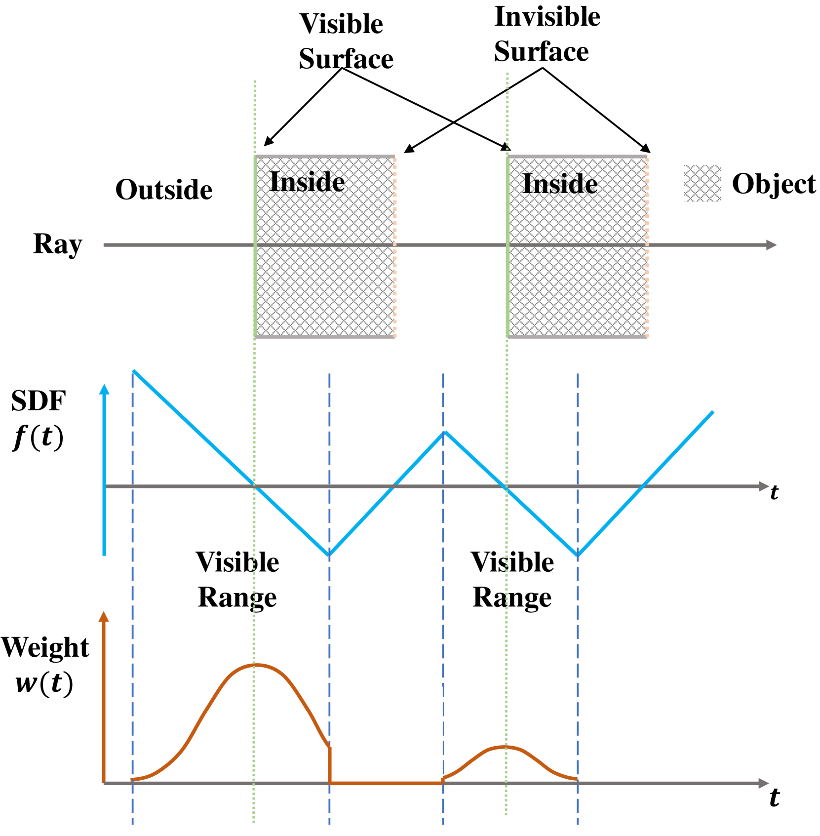
Figure 3: Illustration of weight distribution in case of multiple surface intersection. 不透明度密度函數會改寫成 Eq. \eqref{eq:10}:
$$ \begin{equation} \begin{aligned} \rho(t) = \max\left( \frac{-\frac{-\mathrm{d}\Phi_s}{\mathrm{d}t} \left( f(\mathbf{p}(t)) \right)}{\Phi_s (f(\mathbf{p}(t)))}, 0 \right). \end{aligned} \tag{10} \label{eq:10} \end{equation} $$有了這個方程式,就能使用標準 volume rendering 來計算 weight function。
作者通過推導證明,使用 Eq. \eqref{eq:5} 與 Eq. \eqref{eq:10} 進行 volume rendering 是 unbiased 的。即 weight function 會在第一個表面達到最大值。(推導過程在補充資料)
Discretization#
作者採用與 NeRF 相同的離散化策略,從相機原點延射線採樣,來近似光線的像素顏色:
$$ \begin{equation} \hat{C} = \sum_{i=1}^{n} T_{i} \alpha_i c_i, \tag{11} \end{equation} $$$T_i$ 是離散累積透射率:
$$ \begin{equation*} T_i = \prod_{j=1}^{i-1} (1 - \alpha_j), \end{equation*} $$$\alpha_i$ 離散不透明度:
$$ \begin{equation} \begin{aligned} \alpha_i = 1 - \exp\left( - \int_{t_i}^{t_{i+1}} \rho(t) \, \mathrm{d}t \right), \end{aligned} \tag{12} \end{equation} $$可以進一步得到 (推導過程在補充資料):
$$ \begin{equation} \begin{aligned} \alpha_i = \max\left( \frac{\Phi_s(f(\mathbf{p}(t_i))) - \Phi_s(f(\mathbf{p}(t_{i+1})))}{\Phi_s(f(\mathbf{p}(t_i)))}, 0 \right). \end{aligned} \tag{13} \end{equation} $$Training#
Loss Function#
Total Loss
$$ \begin{equation} \begin{aligned} \mathcal{L} = \mathcal{L}_{color} + \lambda \mathcal{L}_{reg} + \beta \mathcal{L}_{mask}. \end{aligned} \tag{14} \end{equation} $$Color Loss (R is L1 Loss)
$$ \begin{equation} \begin{aligned} \mathcal{L}_{color} = \frac{1}{m} \sum_k \mathcal{R}(\hat{C}_k, C_k). \end{aligned} \tag{15} \end{equation} $$Eikonal Regularization
用來正規化 SDF
$$ \begin{equation} \begin{aligned} \mathcal{L}_{reg} = \frac{1}{nm} \sum_{k,i} \left(\| \nabla f(\mathbf{\hat{p}}_{k,i}) \|_2 - 1\right)^2. \end{aligned} \tag{16} \end{equation} $$Mask Loss (optional)
$$ \begin{equation} \begin{aligned} \mathcal{L}_{mask} = \text{BCE}(M_k, \hat{O}_k), \end{aligned} \tag{17} \end{equation} $$$$ \begin{align*} \hat{O}_k = \sum_{i=1}^{n} T_{k,i} \alpha_{k,i} \end{align*} $$
Hierarchical Sampling#
與 NeRF 的方法不一樣的是,NeRF 使用 coarse network 和 fine network。
本篇只有使用一個網路。 coarse sampling 的機率是通過固定的標準差的 S-density 算出來的,而 fine sampling 是通過可學習的 $s$ 的 S-density 計算得到。
Experiments#
Experimental Settings#
- Datasets
- DTU
- BlenderMVS
- Metrics
- Chamfer distances
- Baselines
- IDR
- DVR
- NeRF
- COLMAP
- UNISURF
Implementation Details#
- Sample 512 rays per batch.
- 300k iterations.
- Training time
- 14 hours (for the ‘w/ mask’ setting)
- 16 hours (for the ‘w/o mask’ setting)
- A single NVIDIA RTX 2080Ti GPU.
- Model the background by NeRF++.
Comparisons#
作者在兩種設定下作比較:
- 有 mask 監督
- 無 mask 監督
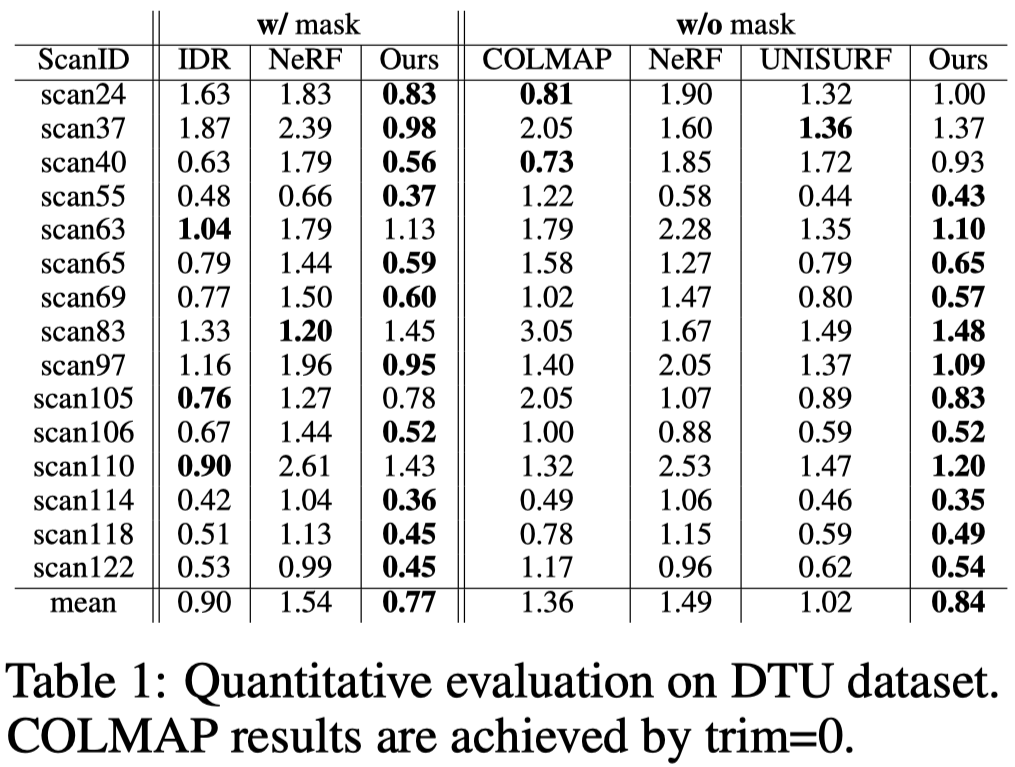
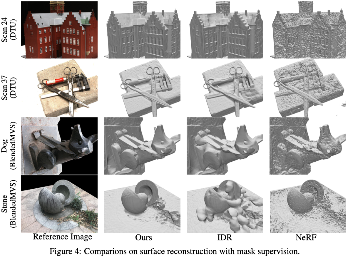
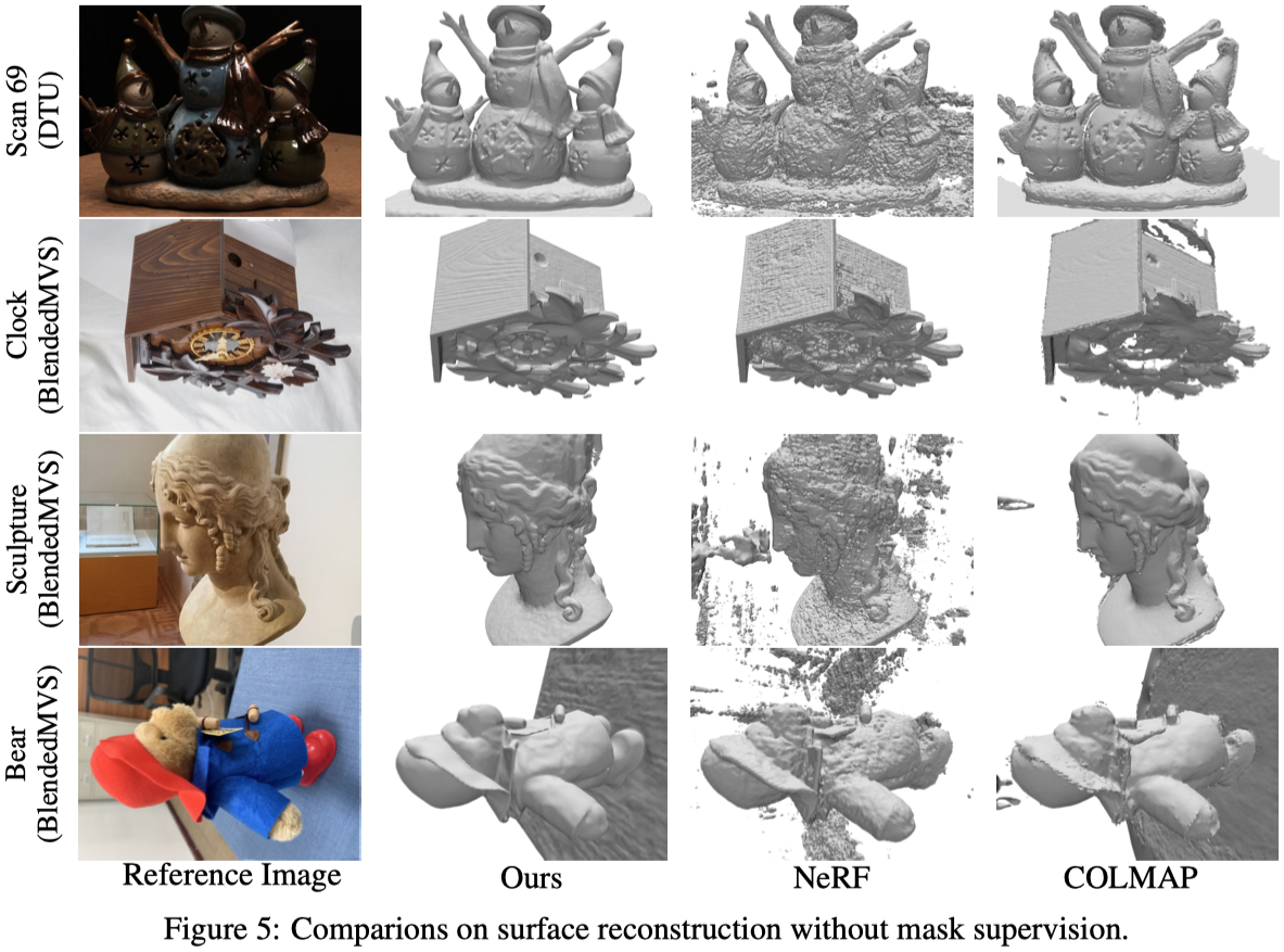
Fig.4 和 Fig.5 展示兩種設定下的可視化結果。
在使用遮罩監督的方法下, IDR 在 DTU Scan 37 中重建薄金屬零件的能力有限,也無法重建 BlenderMVS Stone 中深度有巨大落差的物體。
而 NeRF 因為對於 3D 幾何形狀沒有足夠的約束,因此其提取的網格是嘈雜的。
Analysis#
Ablation Study#
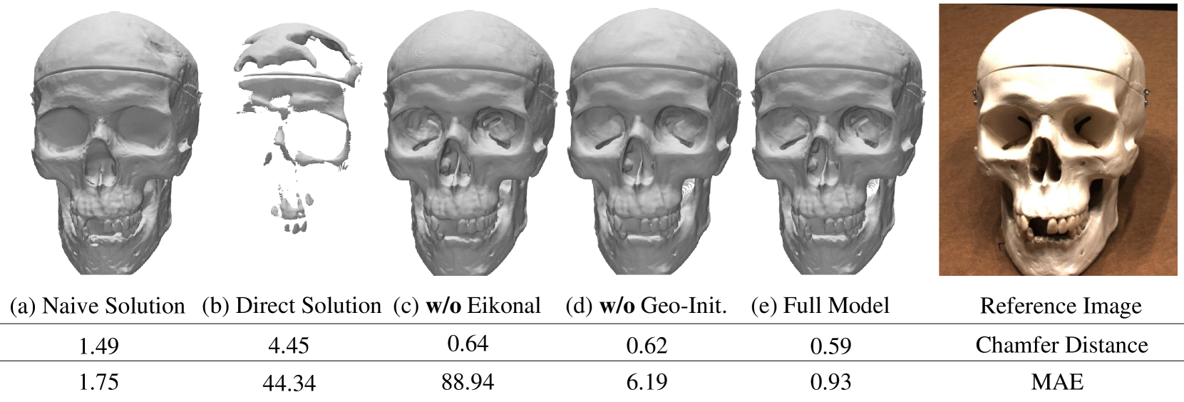
(a) Naive Solution: 會給表面重建帶來 bias。
(b) Direct Solution: 考慮了 unbiased ,但沒有遮擋感知,會帶來嚴重的偽影。
作者也測試了 Eikonal regularization 和 geometric initialization。當沒有這兩項,即使 Chamfer distances 與 full model 相似,但他們無法輸出正確的 SDF。(MAE 很大)
Thin Structures#
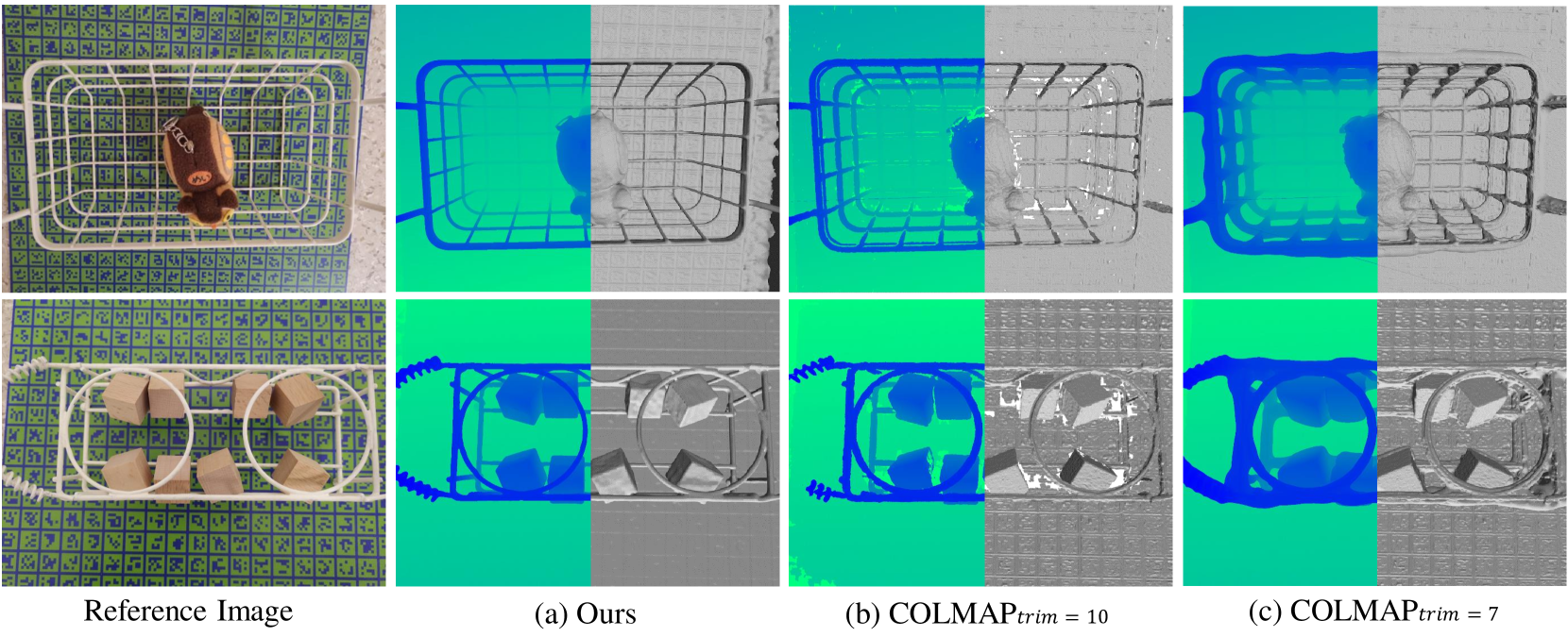
作者另外挑選了兩個具有挑戰性的薄物體。
本篇的方法能夠準確的重建這些薄結構,也能處理薄結構和一般物體混和的場景。
Conclusion#
- 提出 NeuS,一種多視圖表面重建的新方法,將 3D 表面表示為神經 SDF。
- 開發一種新的 volume rendering 方法來訓練隱式 SDF 表示。
- NeuS 能夠產生高品質的重建並成功重建具有嚴重遮蔽和複雜結構的物體,效果超過 SOTA。
Limitation#
- 對於無紋理的物體,性能可能會下降。
- 由於 NeuS 只使用一個尺度參數 $s$ 來對整個空間進行建模,因此當物體的空間位置差異較大,性能可能會下降。