
本篇筆記為筆者在閱讀 HumanNeRF (CVPR 2022) 這篇論文時的隨記。該研究提出了一種方法,用於從單眼視角的影片(monocular video)中,為移動中的人物生成自由視角的渲染結果。這項技術試圖解決在僅有單一、變動視角輸入的情況下,重建人物在任意新視角下的外觀(包含姿態、衣物等細節)的挑戰。筆記將整理 HumanNeRF 的核心方法,包括如何使用標準體積表示(canonical volume)、分解運動場(motion field decomposition),以及姿態修正(pose correction)等技術來實現其目標。
論文資訊
- Link: https://arxiv.org/abs/2201.04127
- Conference: CVPR 2022
Introduction#
- 介紹 HumanNeRF:
- 針對展示複雜動作的人類的單眼視頻的自由視點渲染方法(例如,YouTube 影片)。
- 允許在任何幀上暫停並從新的攝像機視角或該幀和姿勢的 360 度攝像機路徑進行渲染。
- 挑戰:
- 從各種攝像機角度(包括未見角度)合成真實感的細節。
- 合成像衣物摺痕和面部外觀等細節。
- Problems:
- 希望在任何幀上暫停並環繞表演者旋轉 360 度以從任何角度查看。
- 由於需要合成未見的攝像機視角並考慮各種詳細動作,自由視點渲染是一個長期的挑戰。
- Previous works:
- 通常假定多視圖輸入或仔細的實驗室捕捉,並且由於非剛性身體運動而在人類上表現不佳。
- 針對人類的方法通常使用 SMPL 模板,這導致在衣物和複雜動作中產生 artifacts。
- 可變形 NeRF 方法對小變形表現良好,但對大型、全身動作(如舞蹈)表現不佳。
- Methodology:
- HumanNeRF 採用單個視頻,進行每幀分割和自動 3D 姿勢估計,然後優化 canonical, volumetric T-pose。
- Motion field 通過 backward warping 將 canonical volume 映射到每個視頻幀,結合骨架剛性和非剛性運動。
- Data-driven solution,針對大型身體變形進行優化,包括 3D pose refinement 的端到端訓練,無 template models。
- Results:
- 在各種示例上展示:現有的實驗室數據集、實驗室外捕獲的視頻和 YouTube 下載(經創作者許可)。
- Outperforms tate-of-the-art,並產生顯著更高的視覺質量。
Methods#
Overview#
Representing a Human as a Neural Field#
本篇中,作者以一個 canonical appearance volume $F_c$ 來呈現移動的人,並將其扭曲至 observed pose,以產生 output appearance volume $F_o$:
$$ \begin{equation} F_o(\mathbf{x}, \mathbf{p}) = F_c(T(\mathbf{x}, \mathbf{p})), \tag{1} \end{equation} $$where,
- $F_c : \mathbf{x} \rightarrow (c, \sigma)$ maps position $\mathbf{x}$ to color $\mathbf{c}$ and density $\sigma$。
- $T : (\mathbf{x}_o, \mathbf{p}) \rightarrow \mathbf{x}_c$ defines a motion field mapping points from observed space back to canonical space, guided by observed pose
- $\mathbf{p} = (J, \Omega)$: observed pose
- $J$ includes $K$ standard 3D joint locations
- $\Omega = \{ \omega_i\}$ are local joint rotations represented as axis-angle vectors $\omega_i$
作者將 motion field 分解成兩個部分,來更好的建模具有複雜變形的人體動作。
$$ \begin{equation} T(\mathbf{x}, \mathbf{p}) = T_{\text{skel}}(\mathbf{x}, \mathbf{p}) + T_{\text{NR}}(T_{\text{skel}}(\mathbf{x}, \mathbf{p}), \mathbf{p}), \tag{2} \label{eq:2} \end{equation} $$where,
- $T_{\text{skel}}$ represents skeleton-driven deformation, essentially inverse (volumetric) linear-blend skinning
- $T_{\text{NR}}$ starts from the skeleton-driven deformation and produces an offset $\Delta \mathbf{x}$ to it
對於野外場景,作者使用現成的 3D body+camera pose estimator (SPIN)。
因為不準確的 pose estimation,作者也使用了一個 pose correction function $P_{\text{pose}}(\mathbf{p})$ 來更好的解釋 observation,並改善 skeleton-driven deformation。 作者將 Eq.\ref{eq:2} 中的 $T_{\text{skel}}(\mathbf{x}, \mathbf{p})$ 以 $T_{\text{skel}}(\mathbf{x}, P_{\text{pose}}(\mathbf{p}))$ 取代。
Canonical volume#
作者利用一個 MLP 將 canonical volume $F_c$ 表示成一個 continuous field:
$$ \begin{equation} F_c(\mathbf{x}) = \text{MLP}_{\theta_c}(\gamma(\mathbf{x})), \tag{3} \end{equation} $$where,
$\gamma$ is a sinusoidal positional encoding
$L$ is a hyper-parameter that determines the number of frequency bands [41]
Skeletal motion#
根據 Vid2Actor,作者計算的 skeletal deformation $T_{\text{skel}}$ 是一種 inverse, linear blend skinning 的方式,將 observation space 中的點映射到 canonical space:
$$ \begin{equation} T_{\text{skel}}(\mathbf{x}, \mathbf{p}) = \sum_{i=1}^{K} w^i_o(\mathbf{x}) (R_i \mathbf{x} + t_i), \tag{4} \end{equation} $$where,
- $w^i_o$ is the blend weight for the $i$-th bone
- $R_i, t_i$ are the rotation and translation, respectively, that map the bone’s coordinates from observation to canonical space. $R_i$ and $t_i$ can be explicitly computed from $\mathbf{p}$ (see supplementary).
關於 skeletal motion 的點映射,詳細內容寫在補充資料的 「A. Derivation of Motion Bases」
首先定義 body pose $\mathbf{p} = (J, \Omega)$,其中 $J = \{j_i\}$ 包含 $K$ 個關節位置,$\Omega = \{ \omega_i \}$ 為使用 axis-angle representations $\in \mathcal{so}(3)$ 表示的 local joint rotations。
給定預先定義的 canonical pose $\mathbf{p}_c = ( J^c, \Omega^c )$ 與 observed pose $\mathbf{p} = (J, \Omega)$,對於 body part $k$ 的 observation-to-canonical transformation $M$ 為 Eq.\ref{eq:16}:
$$ \begin{equation} M_k(\mathbf{p}_c, \mathbf{p}) = \prod_{i \in \tau(k)} \begin{bmatrix} \exp(\omega^c_i) & j^c_i \\ 0 & 1 \end{bmatrix} \left\{ \prod_{i \in \tau(k)} \begin{bmatrix} \exp(\omega_i) & j_i \\ 0 & 1 \end{bmatrix} \right\}^{-1} \tag{16} \label{eq:16} \end{equation} $$where,
- $\exp(\omega) \in SO(3)$ is a $3 \times 3$ rotation matrix computed by taking the exponential of $\omega$ (i.e., applying Rodrigues’ rotation formula)
- $\tau(k)$ is the ordered set of parents of joint $K$ in the kinematic tree
最後, 對於 body part $k$ 的 rotation $R_k$ 與 translation $t_k$ 可以通過 Eq.\ref{eq:17} 從 $M_k$ 中提取:
$$ \begin{equation} \begin{bmatrix} \mathbf{R}_k & \mathbf{t}_k \\ 0 & 1 \end{bmatrix} = M_k(\mathbf{p}_c, \mathbf{p}) \tag{17} \label{eq:17} \end{equation} $$在實作上,作者通過儲存一組體積 $\{ w_c^i (\mathbf{x})\}$ 作為 $K$ 個 blending weight 來求解定義在 canonical space 中的 $w_c^i$,從中得到的 observation weights 是:
$$ \begin{equation} w^i_o(\mathbf{x}) = \frac{w^i_c(R_i \mathbf{x} + t_i)}{\sum_{k=1}^{K} w^k_c(R_k \mathbf{x} + t_k)}, \tag{5} \label{eq:5} \end{equation} $$在 canonical space 中求解一組的 weight volumes $\{ w_c^i (\mathbf{x})\}$ 可以達到更好的泛化效果,而不是 $N$ 組 $\{ w_o^i (\mathbf{x})\}$ ,因為它能夠避免 overfitting 的問題。
作者將一組 $\{ w_o^i (\mathbf{x})\}$ 打包成一個具有 $K$ 通道的 volume $W_c(\mathbf{x})$。不通過 MLP 而是直接使用顯式 volume representation 的原因有二:
- Eq.\ref{eq:5} 中顯示,當要計算每個 $w_o^i (\mathbf{x})$ 時需要 $K$ 個 MLP,這樣對於優化很沒效率 ($K$ = 24 in our work)
- 通過三線性插值重新取樣的具有有限解析度的顯式體積提供了平滑性,這可以幫助後期的優化規範化。
實作上,並不會直接解出 $W_c$,而是通過一個 CNN ,並輸入一個 random (constant) latent code $\mathbf{z}$ 來得到:
$$ \begin{equation} W_c(\mathbf{x}) = \text{CNN}_{\theta_{\text{skel}}}(\mathbf{x}; \mathbf{z}), \tag{6} \end{equation} $$作者同時多加了一個通道(background class),因此 $W_c$ 有 $K+1$ 個通道。接著作者在 CNN 的輸出使用 channel-wise softmax,來強制跨通道的統一劃分。
在 Eq.\ref{eq:5} 中,分母 ($\sum_{k=1}^{K} w^k_c(R_k \mathbf{x} + t_k)$) 可以看作近似物體部分的 likelihood $f(\mathbf{x})$。如果 $f(\mathbf{x})$ 趨近於零,則表示這個點可能在 free space 中。這個概念會在後面 volume rendering 的部分使用到。
Non-rigid motion#
作者將 non-rigid motion $T_{\text{NR}}$ 表示成 skeleton-driven motion 的一個 offset $\Delta \mathbf{x}$:
$$ \begin{equation*} \Delta \mathbf{x}(\mathbf{x}, \mathbf{p}) = T_{\text{NR}}(T_{\text{skel}}(\mathbf{x}, \mathbf{p}), \mathbf{p}) \end{equation*} $$為了捕捉更多的細節,作者使用 MLP 表示 $T_{\text{NR}}$ (Eq.\ref{eq:7}):
$$ \begin{equation} T_{\text{NR}}(\mathbf{x}, \mathbf{p}) = \text{MLP}_{\theta_{\text{NR}}}(\gamma(\mathbf{x}); \Omega), \tag{7} \label{eq:7} \end{equation} $$Pose correction#
從圖像估計的 body pose 可能不準確,因此作者通過 Eq.\ref{eq:8} 來更新 (修正) pose:
$$ \begin{equation*} P_{\text{pose}}(\mathbf{p}) = (J, \Delta_\Omega(\mathbf{p}) \otimes \Omega), \tag{8} \label{eq:8} \end{equation*} $$過程中作者固定 joints $J$,並優化相關的 joint angles。$\Delta_\Omega = (\Delta \omega_0, \dots, \Delta \omega_K)$ 被添加到 $\Omega$ 中來更新 rotation vectors。
作者發現,不是直接優化 $\Delta_\Omega$,而是通過 MLP 根據 $\Omega$ 產生 $\Delta_\Omega$ (Eq.\ref{eq:9}),可以更快收斂:
$$ \begin{equation} \Delta_\Omega(\mathbf{p}) = \text{MLP}_{\theta_{\text{pose}}}(\Omega) \tag{9} \label{eq:9} \end{equation} $$經過 pose correction,最終的 warping function 可寫作 Eq.\ref{eq:10}:
$$ \begin{equation} T(\mathbf{x}, \mathbf{p}) = T_{\text{skel}}(\mathbf{x}, P_{\text{pose}}(\mathbf{p})) + T_{\text{NR}}(T_{\text{skel}}(\mathbf{x}, P_{\text{pose}}(\mathbf{p})), \mathbf{p}) \tag{10} \label{eq:10} \end{equation} $$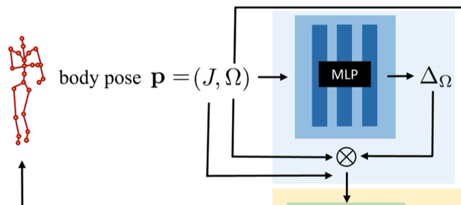
Optimizing a HumanNeRF#
HumanNeRF objective#
給定 input frames $\{I_1, I_2, \ldots, I_N \}$, body poses $\{\mathbf{p}_1, \mathbf{p}_2, \ldots, \mathbf{p}_N \}$ 與 cameras $\{\mathbf{e}_1, \mathbf{e}_2, \ldots, \mathbf{e}_N \}$,本篇模型的優化目標為 Eq.\ref{eq:11},也就是最小化所有網路參數 $\Theta = \{\theta_c, \theta_{\text{skel}}, \theta_{\text{NR}}, \theta_{\text{pose}} \}$ 的 loss。
$$ \begin{equation} \underset{\Theta}{\text{minimize}} \sum_{i=1}^{N} \mathcal{L}\{\Gamma [F_c(T(\mathbf{x}, \mathbf{p}_i)), \mathbf{e}_i], I_i\}. \tag{11} \label{eq:11} \end{equation} $$where,
- $\mathcal{L}(\cdot)$ is the loss function
- $\Gamma[\cdot]$ is a volume renderer
Volume rendering#
每個射線的期望顏色 $C(\mathbf{R})$ 會通過 volume rendering (Eq.\ref{eq:12}) 求得:
$$ \begin{align*} C(r) &= \sum_{i=1}^{D} \left( \prod_{j=1}^{i-1} (1 - \alpha_j) \right) \alpha_i c(\mathbf{x}_i) \tag{12} \label{eq:12} \\ \alpha_i &= 1 - \exp(-\sigma(\mathbf{x}_i) \Delta t_i) \end{align*} $$where,
- $\Delta t_i$ is the interval between sample $i$ and $i+1$
當 approximate foreground probability $f(\mathbf{x})$ 很小時,作者進一步擴增 $\alpha_i$ 的定義如 Eq.\ref{eq:13} 所示:
$$ \begin{equation} \alpha_i = f(\mathbf{x}_i)(1 - \exp(-\sigma(\mathbf{x}_i) \Delta t_i)) \tag{13} \label{eq:13} \end{equation} $$作者使用了原始 NeRF 中提出的 stratified sampling approach 來進行採樣。
Delayed optimization of non-rigid motion field#
當作者使用 Eq.\ref{eq:11} 來優化網路時發現,skeleton-driven 與 non-rigid motions 在優化過程中並沒有完全拆解 (受試者的一部分骨架運動由非剛性運動場建模 )。這是因為非剛性運動對輸入圖像的過度擬合。因此,在渲染未見過的視角時,品質會降低。
作者通過調整優化過程來解決這個問題。
具體來說,作者在優化開始時禁用非剛性運動,然後在後續的過程中以由粗到細的方式逐步重新引入它們 。對於非剛性運動的 MLP,作者應用了 truncated Hann window 到其 position encoding 的 frequency bands 上,以防止對數據的過擬合,並在優化過程中逐步增大窗口的大小。跟隨 Park et al. [47] 的方法,為 position encoding 的每個 frequency band 定義了權重 (Eq.\ref{eq:15}):
$$ \begin{equation} \tau(t) = L \frac{\max(0, t - T_s)}{T_e - T_s} \tag{15} \label{eq:15} \end{equation} $$where,
- $t$ is the current iteration
- $T_s$ and $T_e$ are hyperparameters that determine when to enable non-rigid motion optimization and when to use full frequency bands of positional encoding
此外,作者移除了 position encoding 中的 position identity,其不會影響結果。
Loss and ray sampling#
Loss function#
$$ \begin{equation*} \mathcal{L} = \mathcal{L}_{\text{LPIPS}} + \lambda \mathcal{L}_{\text{MSE}} \end{equation*} $$- LPIPS 的 backbone 為 VGG。
- $\lambda = 0.2$
Patch-based ray sampling#
由於作者使用了 LPIPS 作為 loss function,因此原始 NeRF 的 ray sampling 方法不適用。(LPIPS 會使用 CNN 提取影像特徵)
作者採樣圖片上 $G$ 個尺寸為 $H \times H$ 的 patches ,並渲染每個 batch 總共 $G \times H \times H$ 個射線。模型會將 rendered patch 與輸入影像上相應位置的 patch 進行比較。
Experiments#
Experiment Settings#
Datasets
- ZJU-MoCap
- Self-captured data
- YouTube videos
作者使用 SPIN 來獲得近似的相機和身體姿勢,並自動分割前景主體,然後手動糾正分割中的錯誤。(準確的場景分割 mask 對於渲染品質影響很大)
將拍攝主體的高度保持在約 500 pixels。
Metrics
- PSNR
- SSIM
- LPIPS (VGG)
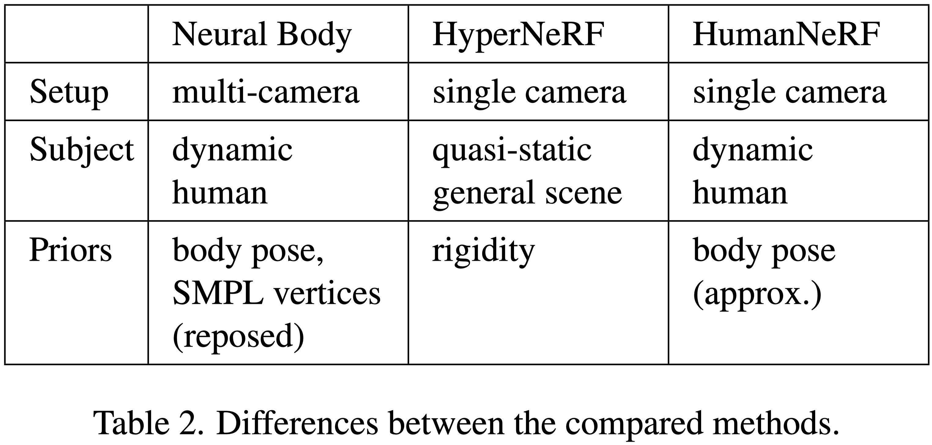
Comparison Targets
Optimization details#
- 128 samples per ray
- 400K iterations (about 72 hours)
- Use 4 GeForce RTX 2080 Ti GPUs
- Delayed optimization
- ZJU-MoCap: $T_s = 10K$ and $T_e = 50K$
- The others: $T_s = 100K$ and $T_e = 200K$ to the others.
- Pose refinement
- ZJU-MoCap: no need
- The others: postpone pose refinement until after $20K$ iterations
Comparisons#
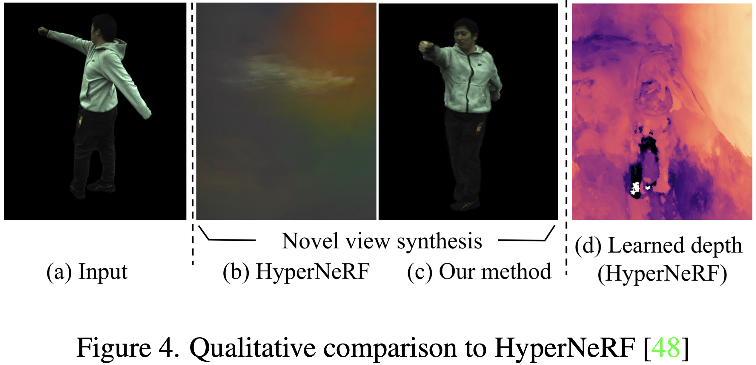
從 Fig.4 中可以看到,HyperNeRF 無法為 novel views 產生有意義的深度圖,作者認為因為 HyperNeRF 依賴 multi-views, 僅僅是將 input view 記起來。此外,動態人體運動也比使用 HyperNeRF 的範例更極端。
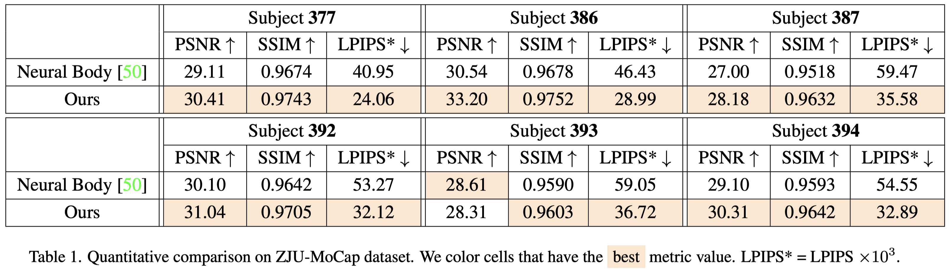
HumanNeRF 在幾乎所有的場景中都比 NeuralBody 表現更好。
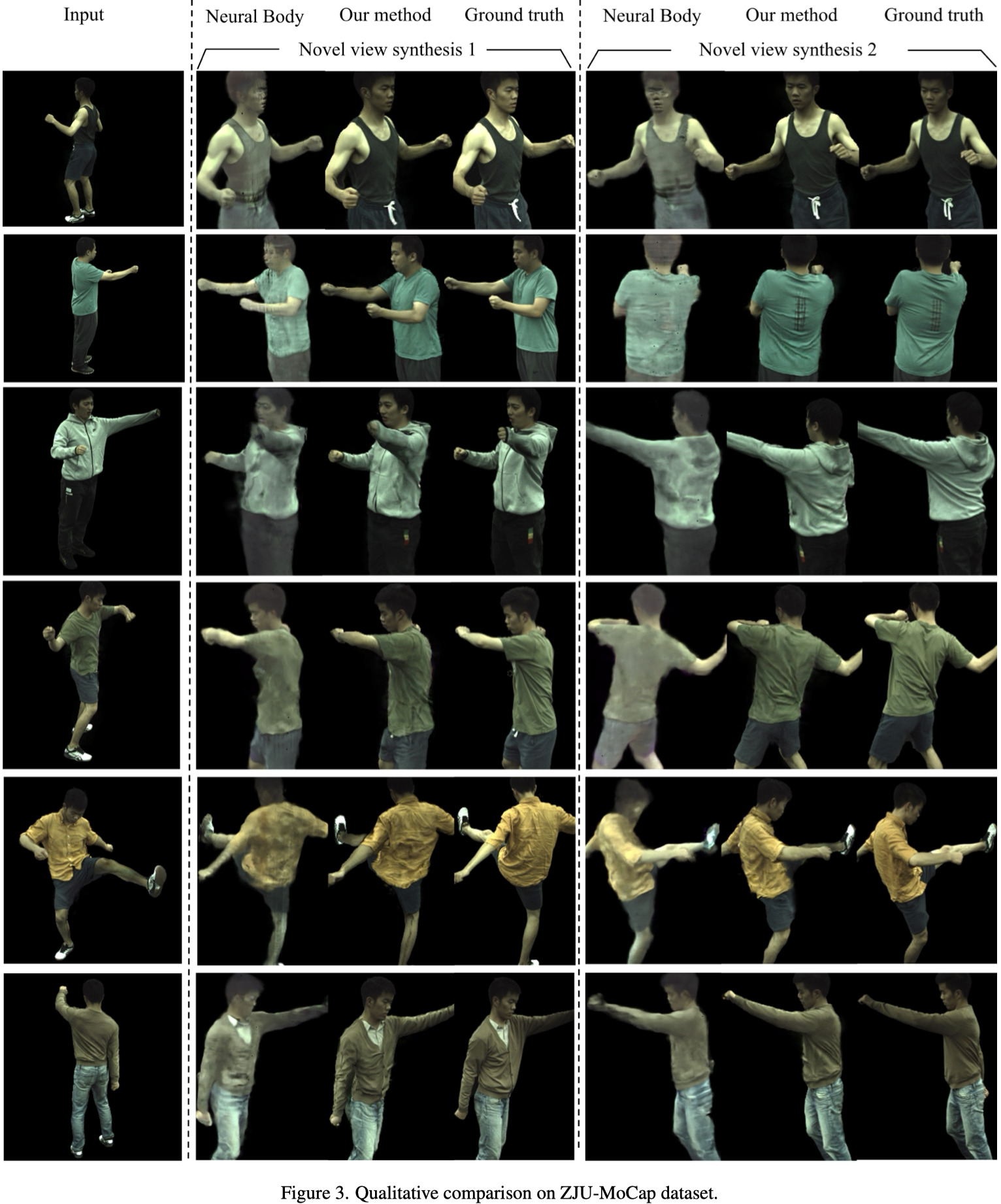
在 Fig.3 中同樣可以看到 HumanNeRF 的渲染品質優於 NeuralBody
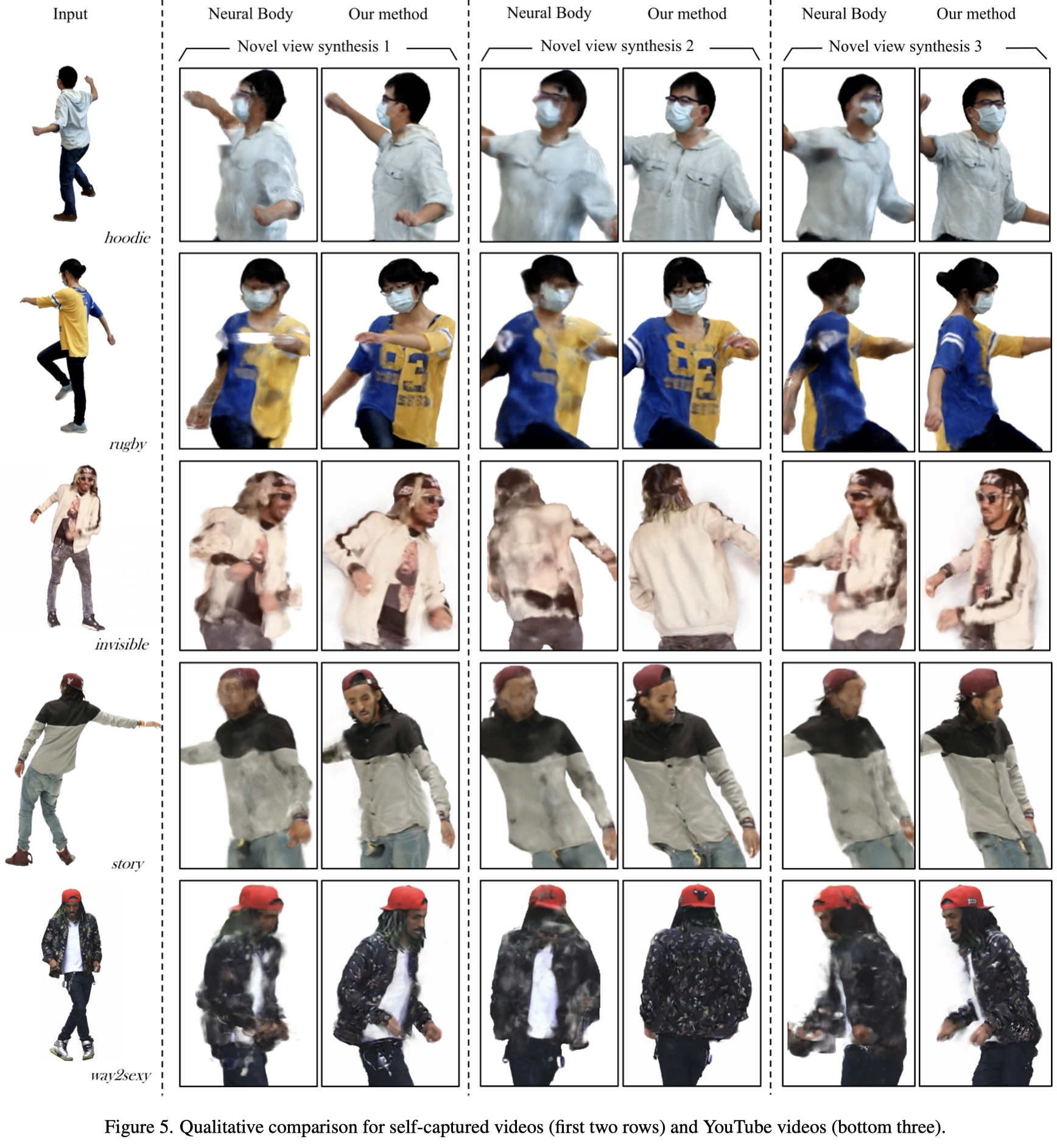
Fig.5 展示了 self-captured 與 YouTube videos 的渲染結果,HumanNeRF 同樣更好。
Ablation studies#
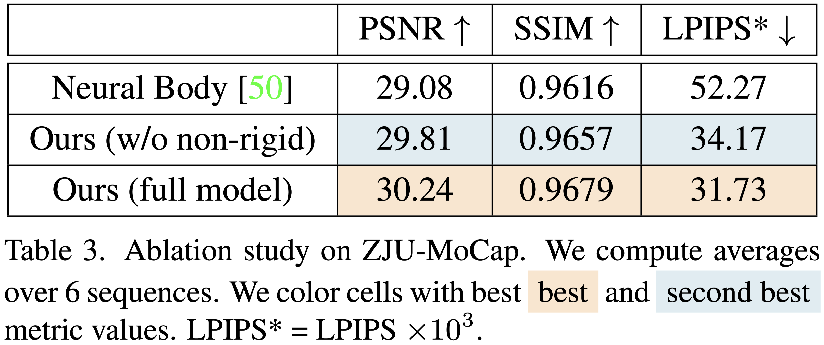
Tab.3 展示,僅使用 skeletal deformation 就能獲得比 NeuralBody 更好的的效果。
加入 non-rigid deformation 後,可以獲得更好的效果。
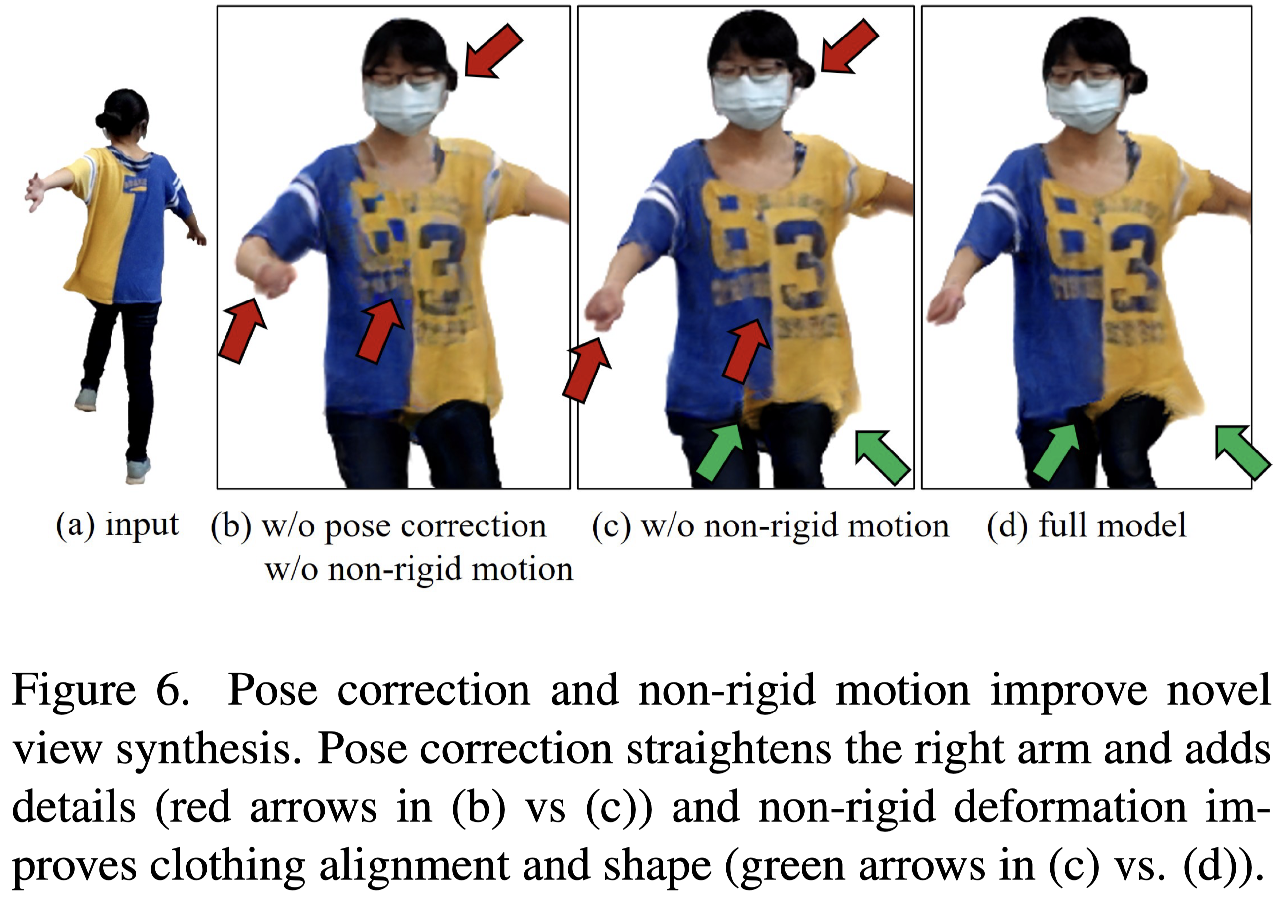
Fig.6 展示了野外場景的可視化效果。從中可以看到 non-rigid motion 的重要性,與 pose correction 對於 unseen view 的重要性。
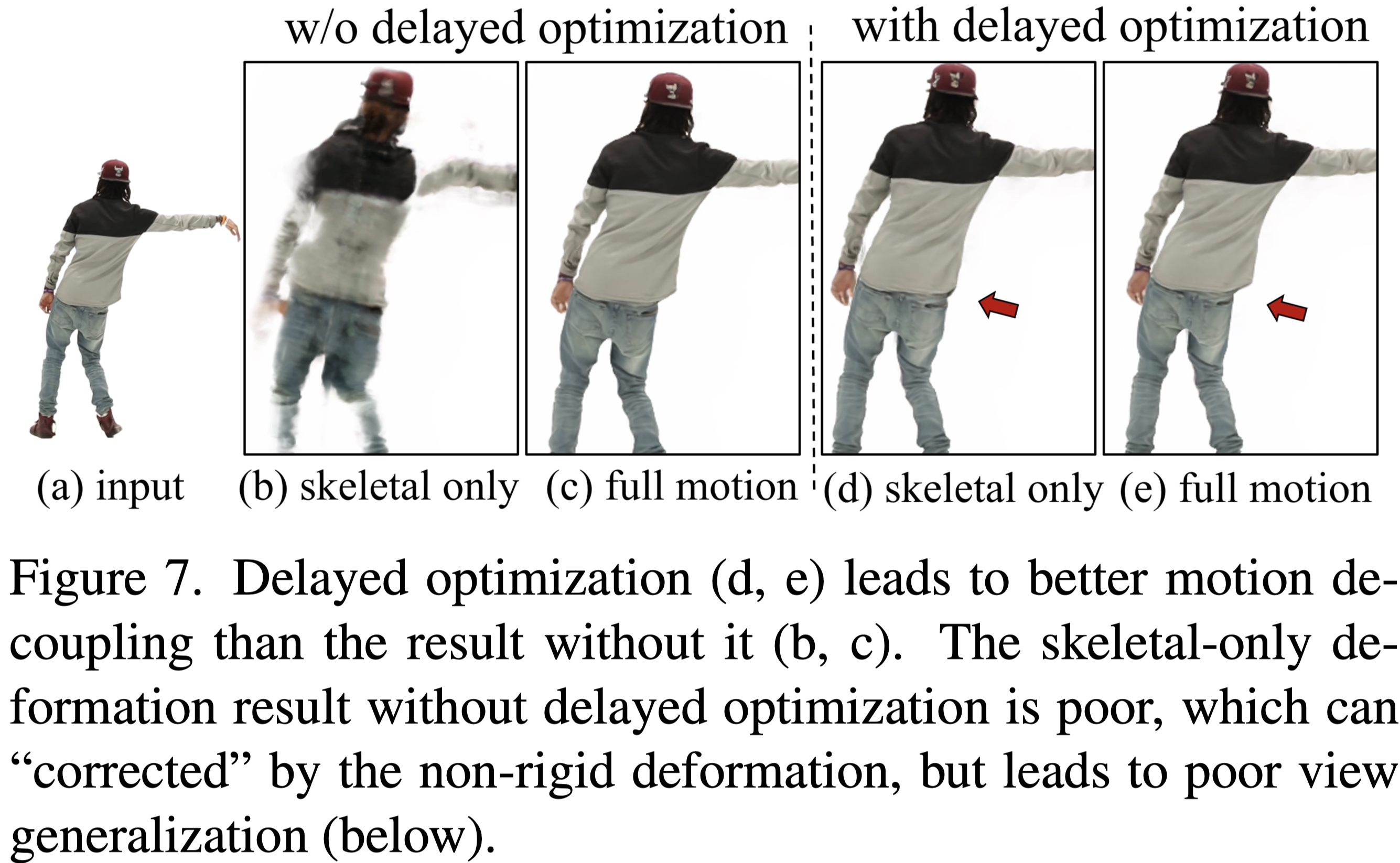
Fig.7 顯示了 delayed optimization 對於解耦 skeletal deformation 與 non-rigid deformation 的重要性。
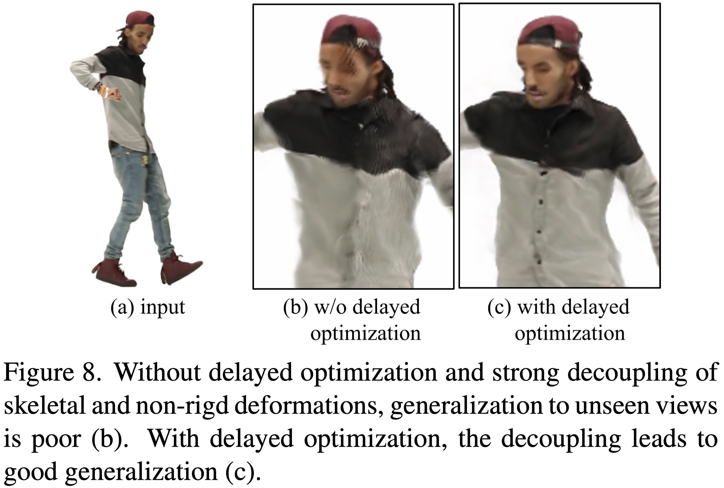
當解耦不好時,對新視圖的泛化會很差,如 Fig.8 所示。
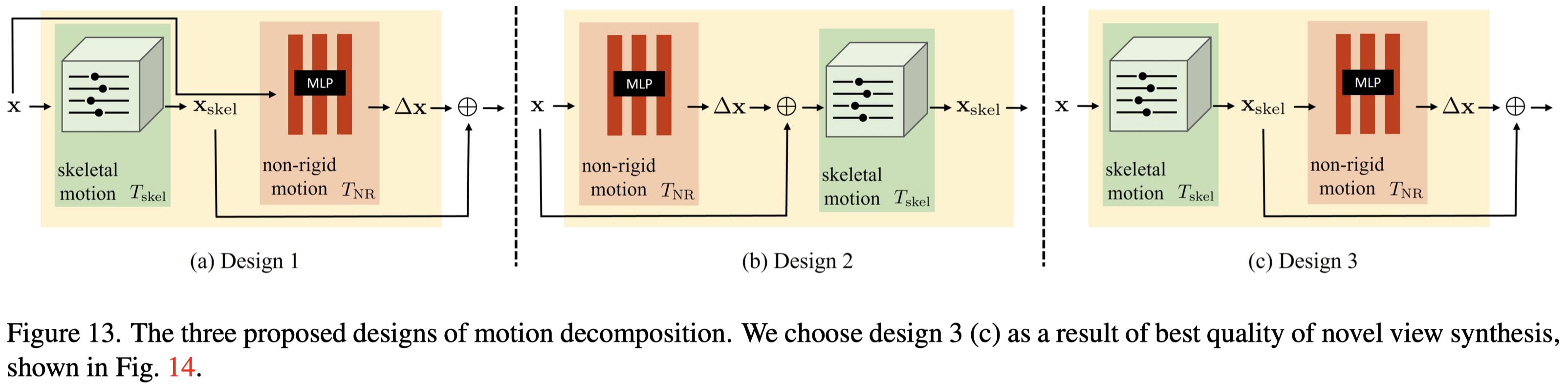
作者另外測試了不同的 Motion Field Decomposition 方案,分別如下:
Design 1 (Eq.\ref{eq:18})
$$ \begin{equation} T(\mathbf{x}) = T_{\text{skel}}(\mathbf{x}) + T_{\text{NR}}(\mathbf{x}) \tag{18} \label{eq:18} \end{equation} $$Design 2 (Eq.\ref{eq:19})
$$ \begin{equation} T(\mathbf{x}) = T_{\text{skel}}(\mathbf{x} + T_{\text{NR}}(\mathbf{x})) \tag{19} \label{eq:19} \end{equation} $$Design 3 (Eq.\ref{eq:20})
$$ \begin{equation} T(\mathbf{x}) = T_{\text{skel}}(\mathbf{x}) + T_{\text{NR}}(T_{\text{skel}}(\mathbf{x})) \tag{20} \label{eq:20} \end{equation} $$
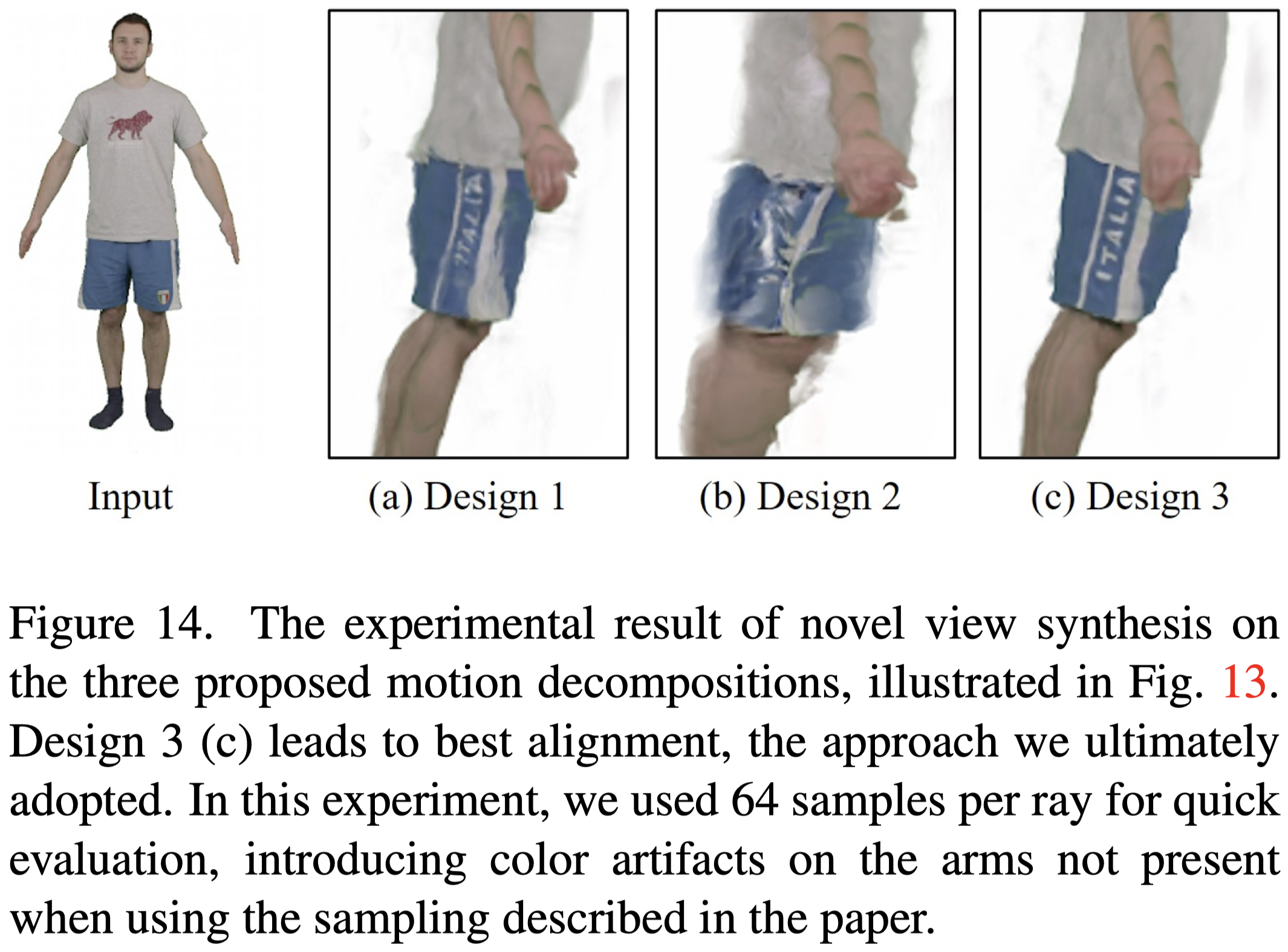
結果顯示 Design 3 的設計方案可以獲得最好的效果。
Conclusion#
- 提出了 HumanNeRF,為單眼影⽚中移動⼈物的⾃由視點渲染提供了最先進的結果。
- 通過仔細建模身體姿勢和運動以及規範化優化過程,我們為這個具有挑戰性的場景展示了高保真度的結果。
Limitations#
- 當影⽚中未顯⽰⾝體的⼀部分時,本篇的⽅法會出現 artifacts。
- 如果初始姿勢估計較差或影像包含嚴重的 artifacts(例如運動模糊),則可能會失敗。
- 即使在姿勢校正之後,逐幀的⾝體姿勢在時間上仍然不平滑。
- 作者假設⾮剛性運動與姿勢相關,但這並不總是正確的。
- 作者假設相當漫射的照明,因此當物件上的點旋轉時,外觀不會發⽣顯著變化。
- 對於野外視頻,需依靠⼿動干預來糾正分割錯誤。