
本篇筆記整理了 DVGO (CVPR 2022) 的研究內容。該論文提出直接體素網格優化方法,針對神經輻射場訓練速度緩慢的問題實現超快收斂。核心技術包括使用密集體素網格建模 3D 幾何體、post-activation 插值技術、兩階段優化策略等。相較於 NeRF 的 10-20 小時訓練時間,DVGO 僅需 15 分鐘即可達到相當品質。
論文資訊
- Link: https://arxiv.org/abs/2111.11215v2
- Conference: CVPR 2022
Introduction#
Previous works:
先前的方法雖然在測試階段有顯著的加速,但只有少數方法實現訓練時間加速,且改進的效果與生成品質較差。
先前使用體素 (voxel grid) 來儲存場景屬性,雖然可以實現實時渲染並產生良好的品質,但缺點是不能從頭開始訓練,需要從訓練好的隱式模型中進行轉換。This paper:
- 本篇加速的關鍵是使用密集的體素網格直接對 3D 幾何體(體積密度)建模。
- Hybrid volumetric representations: 本篇只對顏色使用混合表示(具有淺 MLP 的特徵網格),因精細的顏色策略不在本文的主要範圍內。為了結合 NeRF 的隱式表示和傳統的網格表示,基於坐標的 MLP 被擴展為也以網格中的局部特徵為條件。
- 直接優化密度體素網格會導致超快收斂,但容易出現次優解決方案。本篇使用兩個方法避免:
- 初始化密度體素網格以在任何地方產生非常接近於 0 的不透明度,以避免幾何解決方案偏向相機的近平面。
本偏方法使用梯度下降直接優化體素網格,不依賴神經網路預測網格值。
- 為較少視圖可見的體素提供較低的學習率,這可以避免多餘的體素被分配來解釋少數視角下的觀察結果。
- 初始化密度體素網格以在任何地方產生非常接近於 0 的不透明度,以避免幾何解決方案偏向相機的近平面。
- 由於如何最佳的使用體素網格對體積密度建模仍然是個挑戰,為了簡潔,本篇方法將會使用一個 BBox 將感興趣的區域緊密包圍以分配體素網格。
- Post-activation: 在對密度體素網格進行三線插值後應用所有激活函數。如此可以模擬單個網格單元中的清晰線性表面,因此本篇方法之體素網格僅需要 $160^3$ 即可在多數情況下優於其他方法。
Contribution.
- 實施兩個 pirror 以避免直接優化體積密度時的次優幾何。
- 提出 post-activated voxel-grid interpolation ,使其可以在較低的網格解析度下進行清晰的邊界建模。
- 優點:
收斂速度快兩個量級 (10~20hr v.s. 15min on single 2080ti)。
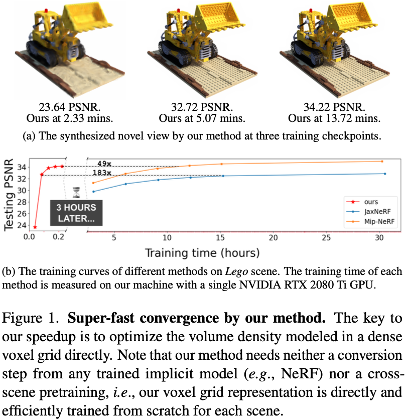
本篇方法不需要跨場景的預訓練。
網格解析度約為 $160^3$,而先前的方法約為 $512^3 \sim 1300^3$。
Methods#
Preliminaries#
MLP
將 NeRF 的 MLP 預測過程表示成 Eq.\ref{eq:1} ,其中省略了可學習的 MLP 參數。
$$ \begin{align*} (\sigma, e) &= \text{MLP}^{(\text{pos})}(x), \tag{1a}\\ c &= \text{MLP}^{(\text{rgb})}(e, d), \tag{1b} \\ \end{align*} \tag{1}\label{eq:1} $$該架構設計來自於 NeRF++
符號 描述 $x$ a 3D position x $d$ a viewing direction $\sigma$ the corresponding density $e$ an intermediate embedding $c$ the view-dependent color emission Position encoding 應用於 $x$ 和 $d$ ,使 MLP 能夠從低維輸入中學習高頻細節。
Output activation.
該架構設計來自於 NeRF++
- 顏色 $c$: $\text{Sigmoid}$
- 密度 $\sigma$: $\text{ReLU}$ or $\text{Softplus}$
Volume rendering
- 根據給定的光學模型,將K個查詢結果累加成具有體繪製正交的單一顏色
符號 描述 $r$ the ray from the camera center through the pixel $K$ the number of points are sampled on $r$ between the pre-defined near and far planes $\alpha_i$ the probability of termination at the point $i$ $T_i$ the accumulated transmittance from the near plane to point $i$ $\delta_i$ the distance to the adjacent sampled point $i$ $c_{bg}$ a pre-defined background color MSE Loss
- 通過最小化 gt color 與 rendered color 之間的 photometric MSE 來訓練模型。
符號 描述 $C(r)$ the observed pixel color $\hat{C}(r)$ the rendered color $\mathcal{R}$ the set of rays in a sampled mini-batch
Post-activated density voxel grid#
- Voxel-grid representation
體素網格表示會在其網格單元中明確地 models 感興趣的模態(如密度、顏色或特徵)。
$$ \begin{align*} \text{interp}(x, V) : \left( \mathbb{R}^3, \mathbb{R}^{C \times N_x \times N_y \times N_z} \right) \to \mathbb{R}^C , \end{align*}\tag{4} $$符號 描述 $x$ the queried 3D point $V$ the voxel grid $C$ the dimension of the modality $N_x \cdot N_y \cdot N_z$ the total number of voxels $\text{interp}$ trilinear interpolation
- Density voxel grid for volume rendering
Density voxel grid ($V^{\text{(density)}}$)是一個特例, $C=1$,用於儲存 volume redering 的密度值。
本篇中的 density activation 使用 Mip-NeRF 中的 $\text{softplus}$
$$ \begin{align*} \sigma = \text{softplus}(\ddot{\sigma}) = \log \left( 1 + \exp(\ddot{\sigma} + b) \right) , \end{align*}\tag{5} \label{eq:5} $$符號 描述 $\ddot{\sigma}$ the raw voxel density before applying the density activation $b$ the shift (hyperparameter) 使用 $\text{softplus}$ 而不是 $\text{ReLU}$ 對直接優化體素密度至關重要,因為當用 $\text{ReLU}$ 作為 density activation 時,體素被錯誤地設置為負值是不可彌補的。反之, $\text{softplus}$ 允許我們探索非常接近 0 的密度。
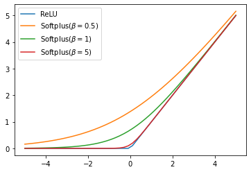
Activation function. - $\text{ReLU}(x) = \max (0, 1)$
- $\text{softplus}{x}=\log (1+\exp(x+\beta))$
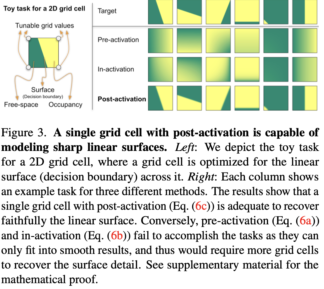
- Sharp decision boundary via post-activation
插值後的體素密度由 softplus 和 alpha 函數 (Eq.\ref{eq:2b}) 依次處理,用於體積渲染:pre-activation, in-activation 與 post-activation。
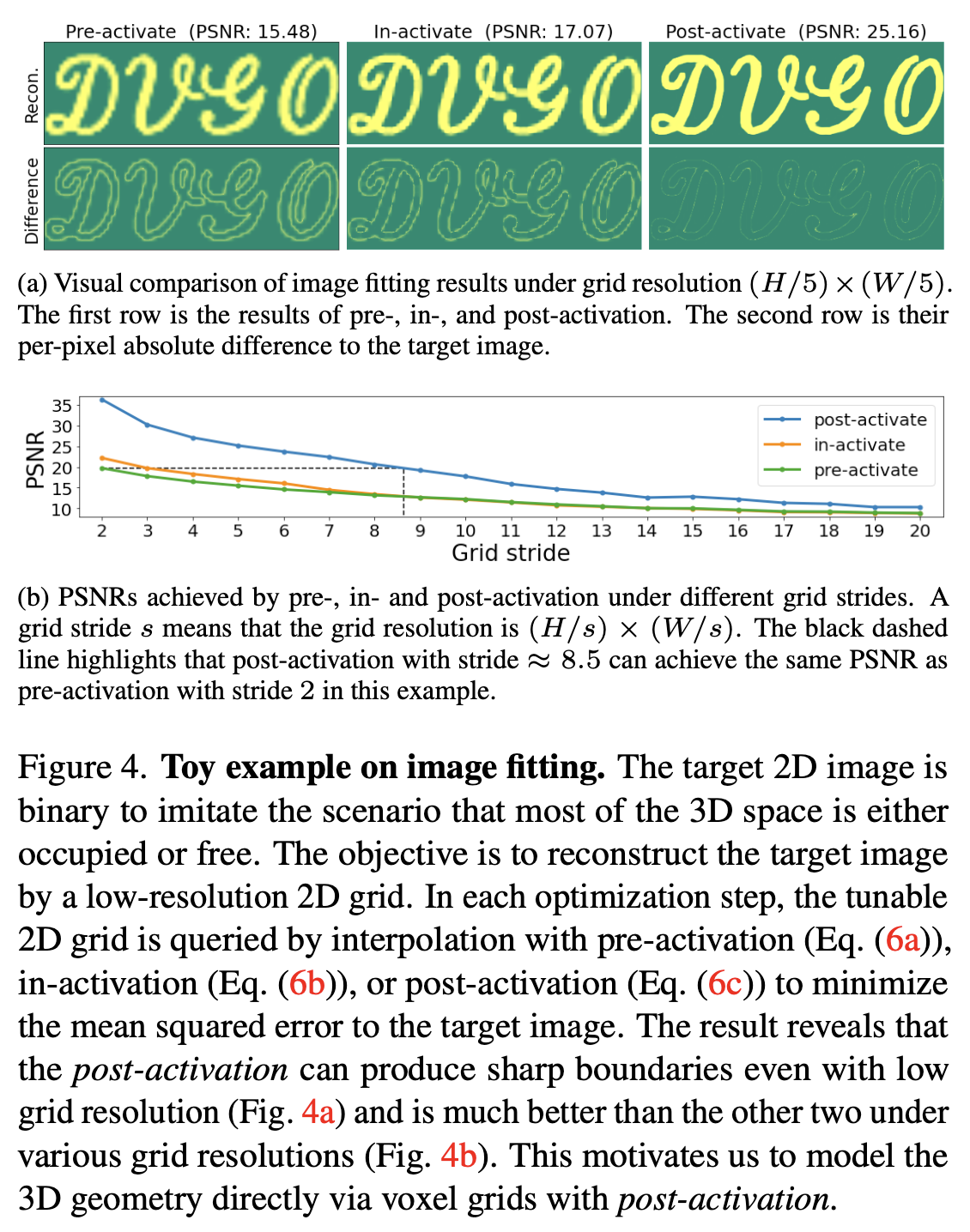
$$ \begin{align*} \alpha^{(\text{pre})} &= \text{interp}\big(x, \text{alpha}(\text{softplus}(V^{(\text{density})}))), \tag{6a} \\ \alpha^{(\text{in})} &= \text{alpha}\big(\text{interp}(x, \text{softplus}(V^{(\text{density})}))), \tag{6b} \\ \alpha^{(\text{post})} &= \text{alpha}\big(\text{softplus}(\text{interp}(x, V^{(\text{density})}))). \tag{6c} \end{align*} $$Post-activation 能夠以更少的網格單元產生清晰的邊界,其餘兩者只能產生平滑的結果。
Toy task for a 2D grid cell
Toy example on image fitting
Fast and direct voxel grid optimization#
在本步驟,將會搜尋場景的粗略幾何,然後再重建包含與 view 相關更精細的細節。
Coarse geometry searching#
通常情況下,一個場景是由 free space(即未定位的空間)主導的。本篇的目標是在重建需要更多計算資源的精細細節和視圖依賴效應之前,有效地找到感興趣的粗略的三維區域。因此,可以在以後的精細階段減少每個射線上的查詢點的數量。
Coarse voxels allocation
- 先找到一個 BBox 緊密包圍 training view 的 camera frustums,接著將 voxel grid 與之對齊。
- The voxel size is $s^{\text{(c)}} = \sqrt[3]{L^{\text{(c)}}_x \cdot L^{\text{(c)}}_y \cdot L^{\text{(c)}}_z / M^{\text{(c)}}}$ ,因此可以得到 $N^{\text{(c)}}_x,N^{\text{(c)}}_y,N^{\text{(c)}}_z = \lfloor L^{\text{(c)}}_x/s^{\text{(c)}} \rfloor,\lfloor L^{\text{(c)}}_y/s^{\text{(c)}} \rfloor,\lfloor L^{\text{(c)}}_z/s^{\text{(c)}} \rfloor$
符號 描述 $L^{\text{(c)}}$ the lengths of the BBox $M^{\text{(c)}}$ the expected total number of voxels $N^{\text{(c)}}$ number of voxels on each side of BBox
Coarse scene representation
使用帶有 post-activation 的 coarse density voxel grid $V^{\text{(density)(c)}} \in \mathbb{R}^{1 \times N^{\text{(c)}}_x \times N^{\text{(c)}}_y \times N^{\text{(c)}}_z}$ 來 model 場景幾何。
只使用 $V^{\text{(rgb)(c)}} \in \mathbb{R}^{3 \times N^{\text{(c)}}_x \times N^{\text{(c)}}_y \times N^{\text{(c)}}_z}$ model view-invariant color emissions。
$$ \begin{align*} \ddot{\sigma}^{(c)} &= \text{interp}(x, V^{(\text{density})(c)}), \tag{7a} \\ c^{(c)} &= \text{interp}(x, V^{(\text{rgb})(c)}), \tag{7b} \end{align*} $$符號 描述 $c^{\text{(c)}} \in \mathbb{R}^3$ the view-invariant color $\ddot{\sigma}^{\text{(c)}} \in \mathbb{R}$ the raw volume density
Coarse-stage points sampling
$$ \begin{align*} x_0 &= o + t^{(\text{near})}d, \tag{8a} \\ x_i &= x_0 + i \cdot \delta^{(c)} \cdot \frac{d}{\lVert d \rVert^2}, \tag{8b} \end{align*} \tag{8}\label{eq:8} $$符號 描述 $o$ the camera center $d$ the ray-casting direction $t^{\text{(near)}}$ the camera near bound $\delta^{\text{(c)}}$ a hyperparameter for the step size $i$ The query index ranges from $1$ to $\lceil t^{\text{(far)}} \cdot \|d\|^2 / \delta^{\text{(c)}} \rceil$ $t^{\text{(far)}}$ the camera far bound Prior 1: low-density initialization
在開始訓練時,由於 Eq.\ref{eq:2c} 中的累積透射率項,遠離攝像機的點的重要性被降低了,而在攝像機附近的平面上密度較高。
必須更仔細地初始化 $V^{\text{(density)(c)}}$,以確保射線上的所有採樣點在開始時對相機可見,累積透射率 $T_is$ 接近於 1。
實作上,作者將 $V^{\text{(density)(c)}}$ 所有的 grid value 初始化為 0,並將 Eq.\ref{eq:5} 中的 bias 項設為 Eq.\ref{eq:9},如此累積透射率 $T_i$ 將衰減至 $1- \alpha^{\text{(init)(c)}}\approx 1$ 。
$$ \begin{align*} b = \log \left( \left( 1 - \alpha^{(\text{init})(c)} \right)^{-\tfrac{1}{s^{(c)}}} - 1 \right) , \end{align*}\tag{9} \label{eq:9} $$符號 描述 $\alpha^{\text{(init)(c)}}$ a hyperparameter $s^{(\text{c})}$ a voxel size
Prior 2: view-count-based learning rate
- 可能有一些體素僅在較少的訓練視圖中可見,然而我們更傾向在許多視圖中具有一致性的表面,而不是一個只能解釋少數視圖的表面。
- 本篇為 $V^{\text{(density)(c)}}$ 中不同的 grid points 設定不同的 learning rate。將基礎的 lr 做 $n_j / n_{\max}$ 的 scale。
符號 描述 $j$ index of each grid point $n_j$ the number of training views which point $j$ is visible $n_{\max}$ the maximum view count over all grid points
Training objective for coarse representation
- Reconstruction loss: MSE
- Regularization loss: background entropy loss.
鼓勵累積的 alpha value 集中在背景或前景上。
Fine detail reconstruction#
給定優化後的粗略幾何 $V^{\text{(density)(c)}}$ ,接著我們可以專注於較小的子空間去重建表面細節與 view-dependent effects。
本階段中, $V^{\text{(density)(c)}}$ 將會被固定。
Known free space and unknown space
作者定義:若 $V^{\text{(density)(c)}}$ 中的 post-activated alpha value 小於 threshod $\tau^{\text{(c)}}$,則將其視為在已知的 free space 中。反之則視為在未知的空間中。Fine voxels allocation
- 密集地查詢 $V^{\text{(density)(c)}}$,以找到一個緊密包圍未知空間的BBox,其中 $L^{\text{(f)}}_x, L^{\text{(f)}}_y, L^{\text{(f)}}_z$ 是 BBox 的長度。
- 唯一的 hyperparameter 是 voxel 的預期總數 $M^{\text{(f)}}$。voxel 大小 $s^{\text{(f)}}$ 和網格尺寸 $N^{\text{(f)}}_x, N^{\text{(f)}}_y, N^{\text{(f)}}_z$ 可以按照第5.1節方法從 $M^{\text{(f)}}$ 中自動得出。
Fine scene representation
使用具有 post-activated interpolation 的 high-resolution density voxel grid $V^{\text{(density)(f)}} \in \mathbb{R}^{1 \times N^{\text{(f)}}_x \times N^{\text{(f)}}_y \times N^{\text{(f)}}_z}$ 。
針對 view-dependent color emission,選擇使用 explicit-implicit hybrid representation,因為顯性表示會造成較差的結果,而隱性表示需要更長的訓練時間。
- A feature voxel grid $V^{\text{(feat)(f)}} \in \mathbb{R}^{D \times N^{\text{(f)}}_x \times N^{\text{(f)}}_y \times N^{\text{(f)}}_z}$ 。
$D$ 是 feature-space dimension 的 hyperparameter。
- A feature voxel grid $V^{\text{(feat)(f)}} \in \mathbb{R}^{D \times N^{\text{(f)}}_x \times N^{\text{(f)}}_y \times N^{\text{(f)}}_z}$ 。
最後給定 $x$ 與 $d$ ,透過 Eq.\ref{eq:10} 計算密度與顏色。
- Position embedding 應用於淺層 MLP 中的 $x$ 與 $d$ 。
符號 描述 $c^{\text{(f)}} \in \mathbb{R}^3$ the view-dependent color emission $\ddot{\sigma}^{\text{(f)}} \in \mathbb{R}$ the raw volume density $\theta$ parameters of MLP
Progressive scaling
- 逐步 scale $V^{\text{(density)(f)}}$ 與 $V^{\text{(feat)(f)}}$。
- 初始 voxels 數量設為 $\lfloor M^{\text{(f)}} / 2^{|\text{pg_chpt}|} \rfloor$,當 training step 達到 $\text{pg_ckpt}$ ,就將 voxels 的數量翻倍,直到最後一個 checkpoint 的 voxel 數量為 $M^{\text{(f)}}$。也就是訓練時 voxel grid 的解析度由小到大。
- 等於說在每個 checkpoint 都會透過三線性插值 resize voxel grids $V^{\text{(density)(f)}}$ 與 $V^{\text{(feat)(f)}}$。
- 逐步 scale $V^{\text{(density)(f)}}$ 與 $V^{\text{(feat)(f)}}$。
Fine-stage points sampling
- 與 Eq.\ref{eq:8} 類似,僅作微調:
- 過濾掉不與已知 free space 相交的射線。
- 將 $t^{\text{(near)}}$ 與 $t^{\text{(far)}}$ 調整為與 ray-box 相交的兩個端點,若 $x_0$ 已經在 BBox 中,則不調整 $t^{\text{(near)}}$。
- 與 Eq.\ref{eq:8} 類似,僅作微調:
Free space skipping
- 由於查詢 $V^{\text{(density)(c)}}$ 比查詢 $V^{\text{(density)(f)}}$ 快,且查詢 view-dependent colors (Eq.\ref{eq:10b}) 最慢,因此將在訓練與測試階段使用 free space skipping 以提升效率。
- 通過檢查 optimized $V^{\text{(density)(c)}}$,跳過處於已知 free space 的採樣點。
- 通過查詢 $V^{\text{(density)(f)}}$ 來跳過在未知 free space 中具有低 activated alpha value (threshold at $\tau^{\text{(f)}}$)
Training objective for fine representation
- 與 coarse stage 一樣的訓練損失,但對於 regularization loss,使用更小的 weight。
Experiments#
Datasets#
- 5 inward-facing datasets
- Synthetic-NeRF、Synthetic-NSVF
- 包含八個由模型合成的具有逼真圖像的物體,兩者的物體不相同。
- 將圖像解析度設為 800×800。
- 讓每個場景有100個視圖用於訓練,200個視圖用於測試。
- Blend-edMVS
- 這是一種合成的多視角立體影像數據集,其中包含了具有真實環境光照的物體模型。
- 使用 NSVF 提供的四個對象的子集。
- 圖片解析度為768×576像素,其中八分之一的圖片用於測試。
- Tanks&Temples
- 一個真實世界的數據集。
- 使用 NSVF 提供的五個場景的子集,每個場景都包含了由一個環繞場景的內向型攝像機拍攝的視圖。
- 圖像解析度為 1920×1080 像素,其中八分之一的圖像用於測試。
- DeepVoxels
- 包含四個簡單的 Lambertian 物體。
Lambertian object: 所有觀察方向看起來均勻明亮並且反射全部入射光的表面。朗伯反射率是理想的無光澤或漫反射表面所表現出的特性。
- 圖像解析度為 512×512。
- 每個場景有 479 個視圖用於訓練,1000 個視圖用於測試。
- 包含四個簡單的 Lambertian 物體。
- Synthetic-NeRF、Synthetic-NSVF
Implementation details#
- 預期的 voxel 數量設為 $M^{\text{(c)}} = 100^3$ 與 $M^{\text{(f)}} = 160^3$。
- The activated alpha value:
- Coarse stage: $\alpha^{\text{(init)(c)}} = 10^{-6}$。
- Fine stage: $\alpha^{\text{(init)(f)}} = 10^{-2}$ ,因為查詢點都集中在優化的粗略幾何上。
- The points sampling step sizes,設置為 voxel sizes 的一半:$\delta^{\text{(c)}} = 0.5 \cdot s^{\text{(c)}}$ 與 $\delta^{\text{(f)}} = 0.5 \cdot s^{\text{(f)}}$ 。
- 淺層 MLP 包含兩個隱藏層,有 128 個 channels。
- 使用 batch size 為 8192 條射線, Adam optimizer 分別以 10k 和 20k 迭代來優化粗略和精細場景表示。
- 所有的 voxel grids 基礎 learning rate 為 0.1,淺層 MLP 為 $10^{-3}$。並使用 exponential learning rate decay。
Comparisons#
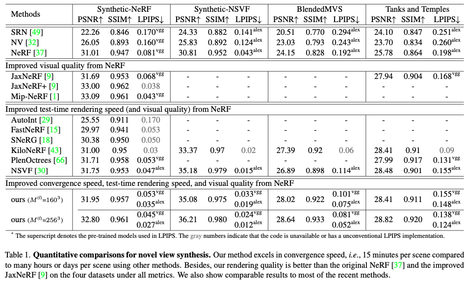
Quantitative evaluation on the synthesized novel view
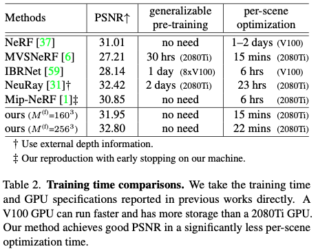
Training time comparisons
Rendering speed comparisons 提升測試時的渲染速度並非本文之關注重點,但仍然在 $800 \times 800$ 的圖像上,與 NeRF 相比實現約 $45\times$的提升 (0.64s v.s 29s)
Qualitative comparison

Ablation studies#
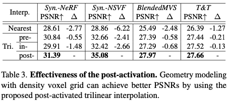
Effectiveness of the post-activation
- 第4節中表明,所提出的後激活三線插值能夠使離散的網格模擬出更清晰的表面。
- 在現實世界捕獲的BlendedMVS和Tanks and Temples數據集中,我們的收穫較少。直觀的原因是,真實世界的數據引入了更多的不確定性(例如,不一致的光照,SfM誤差),這導致了多視角的不一致和更模糊的表面。因此,對於能夠對更清晰的表面進行建模的場景表示來說,其優勢就會減弱。我們推測,在未來的工作中解決不確定性可以增加擬議的後激活的收益。
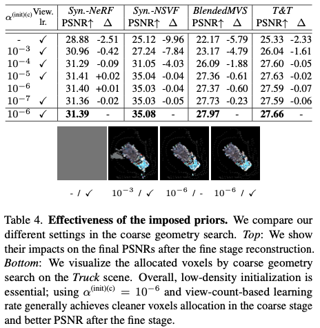
Effectiveness of the imposed priors
Conclusion#
本文介紹了一種基於NeRF的場景重建方法,該方法直接優化體素網格,並實現了與NeRF相當質量的超快收斂速度。